 | 28 Oct 2022
Simple evaluation of the fold axis, axial plane, and interlimb angle from a borehole image log
Yoshinori Sanada
Takehiro Hirose
Folds and fractures are important structures that preserve information on the past stress evolution; however, folds remain largely unexplored. Studying folds remains challenging, as no simple and unified method can be used to evaluate fold parameters, which include the fold axis, axial plane, and interlimb angle with depth. In this study, we propose a method to calculate the fold parameters of cylindrical concentric folds by considering the point at which the bedding trend changes as an inflexion point of the fold. The inflexion point is identified from the analysis of bedding orientation, which can be obtained by borehole image log. The orientation of the fold axis and the axial plane were geometrically calculated based on the inflexion surfaces at both ends of the folds. The application of this method is illustrated using a simulated fold model. It is shown that these fold parameters are calculated using the depth of the fold and are reliable to a certain extent, despite the uncertainty of the inflexion points. Although the extraction method assumes cylindrical concentric folds, it can be applied to symmetric folds to estimate the orientation of the fold axis and axial planes. The method developed in this study is expected to have a wide range of applications in structural geology as it can estimate the fold parameters of each fold traversed by a borehole.
- Article
(7642 KB) - Full-text XML
-
Supplement
(521 KB) - BibTeX
- EndNote


Borehole imaging is a logging technique for the azimuthal surface scan of a borehole wall (Zemanek et al., 1969). It provides information on strikes and dips on features, such as bedding, lithology, grading, fractures, and breakouts. They are utilized in a wide range of geological disciplines including sedimentology, structural geology, metamorphic and volcanic petrology, and geomechanics (e.g. Prensky, 1999). The structural interpretation using stratigraphic orientation data is fundamental for the understanding of the geology around a drilling site. It is a common practice to reconstruct 2D/3D geological structures from the bedding or fracture orientation that is obtained from borehole images and compare them with those obtained by seismic exploration (log-seismic integration; Goldberg, 1997; Moore et al., 2014). Furthermore, geological modelling methods that consider structures such as folds and faults have also been proposed (Etchecopar and Bonnetain, 1992; Etchecopar and Dubas, 1992; Yamada et al., 2016). On the other hand, the resolution of borehole images has developed in recent years, and it is presently possible to recognize sedimentary facies down to a few centimetres. Hence, a borehole can be regarded as a continuous outcrop without the influence of vegetation or topography. This has led to field-like fracture analysis and geological interpretation (Ienaga et al., 2006; Blake and Davatzes, 2012; Lai et al., 2018). However, as for folds, which record past and present stresses, as well as fractures, such mesoscale and outcrop-scale descriptions and analyses have not been commonly performed, which is contrary to the aforementioned extension to large-scale structures.
In borehole images, folded structures are recognized from eye-shaped structures and continuous changes in the orientation of bedding planes on tadpole plots (Vickerman and Spratt, 2011; Crow and Ladevèze, 2015). By extracting this series of changes in orientation and processing statistically on stereographic plotting, the orientations of the fold axes and axial planes can be derived similar to geological outcrop surveys (Holdsworth, 1988). As the eye mark represents the hinge of the fold obliquely aligned with the borehole, it is possible to determine the fold axis azimuth simply by measuring the direction of the eye. Note that this method cannot be used if the hinge line is parallel to the borehole, as the eye mark will not appear. The fold axes, axial planes, and interlimb angles are measured by these methods; however, these methods lack information on the depth of each fold and their spatial variation. Although the small-scale fold is a powerful indicator of the stress orientation (Ramsay and Huber, 1987; Mayer and Albat, 1990; Scott and Selley, 2004), this conventional approach does not focus on their location and is not suitable for investigating local–regional stress evolution. Due to the limited exposure of continuous folds in the field and the measurement of fold parameters being time-consuming, it is important to obtain fold parameters effortlessly in continuous borehole images.
Therefore, this study aims to develop a simple and continuous method for obtaining fold parameters such as the fold axis, axial plane, and interlimb angle based on borehole image data. The proposed method was applied to a folded geological model to examine its effectiveness and feasibility.
The fold structure in the borehole image is observed as a continuous change in the strike and dip of the bedding on the tadpole plot and eye marks (Fig. 1). Although the eye orientation indicates the azimuth of the fold axis and that the axis surface is almost orthogonal to the borehole, the plunge of the axis and the axial plane orientation cannot be obtained. The bedding dip and strike trend on the tadpole plot represent more detailed information on the folds. At the point where one wave of a fold ends and the next one begins (red circle in Fig. 1), the trend of the strike and dip changes. The key to obtaining the fold parameters is to describe this point as the inflexion point of the fold and to identify the inflexion surface at this point. In the case of a symmetric fold, the axial plane is represented as the bisector of the inflexion surface, and the interlimb angle is the angle between two bedding planes at the inflexion point. To formulate them, we consider a cylindrical concentric fold, as shown in Fig. 2. The top of the borehole was set to for simplicity. The borehole and an inflexion point on stratum A of this fold intersect at iA . In addition, another inflexion point on stratum B intersects the borehole at IB . The normal vector of the bedding plane at point iA is n1, and similarly, the normal vector of the bedding at point IB is n2. The normal vector is expressed as follows, using the strike (θ) and dip (ϕ) of the bedding planes at the inflexion points that can be extracted from the borehole image.
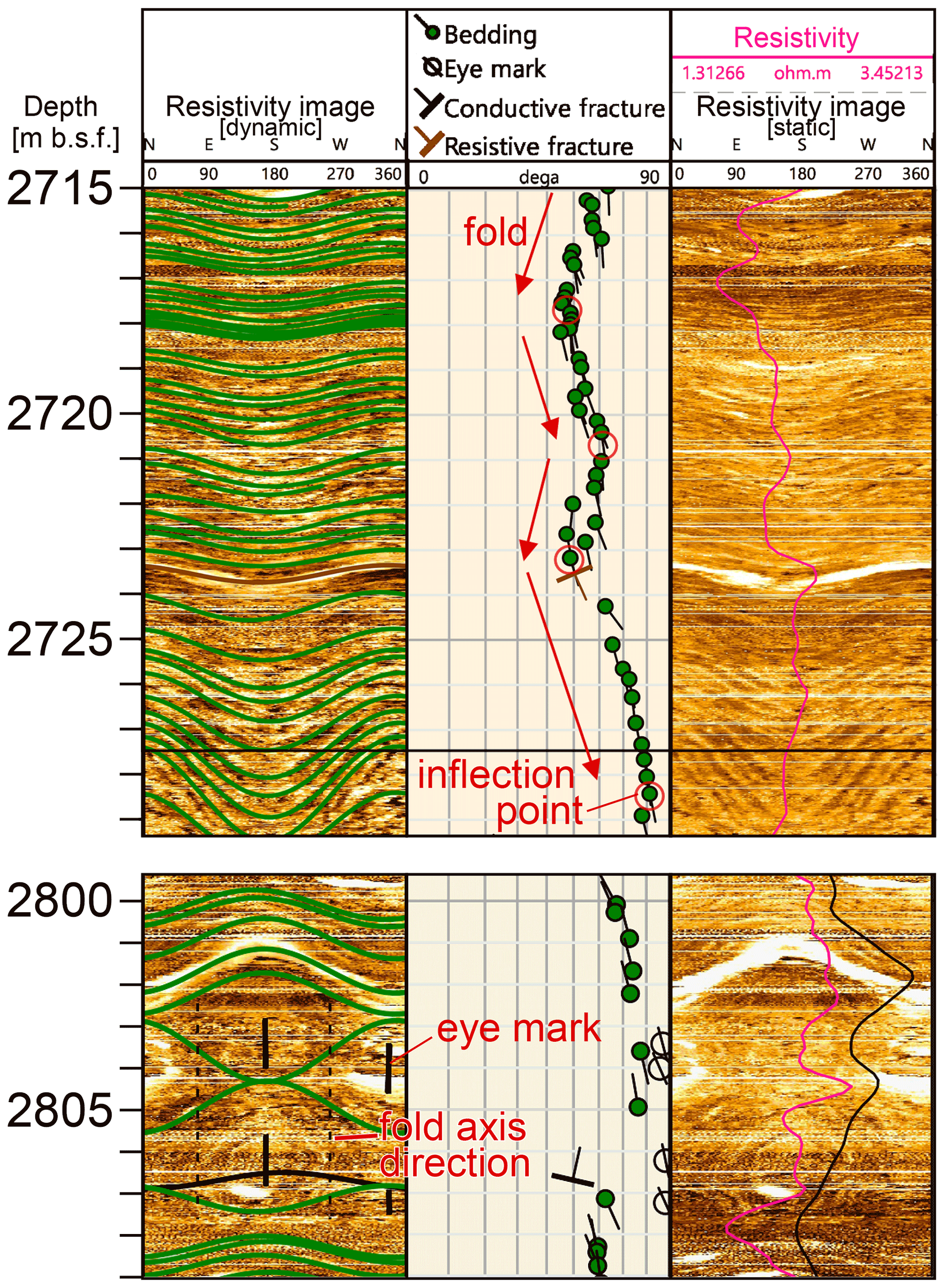
Figure 1Example of fold appearance in a borehole wall image. Bedding planar interpretation, fold inflexion points, and eye marks are interpreted in the electrical resistivity image of the interior of the accretionary complex that was acquired from the IODP (Integrated Ocean Drilling Program) Expedition 348 (Tobin et al., 2015). Green lines in the dynamic resistivity image are fitted using a bedding plane, and its orientations are plotted in tadpole plot. The pink line in the static image is the shallow resistivity value. The folds appear as a systematic increase or decrease in the dip of the bedding. The eye, the hinge of the fold, can also be observed. The orientation of the fold axis is orthogonal to the eye direction and is indicated by the dotted line in the lower column.
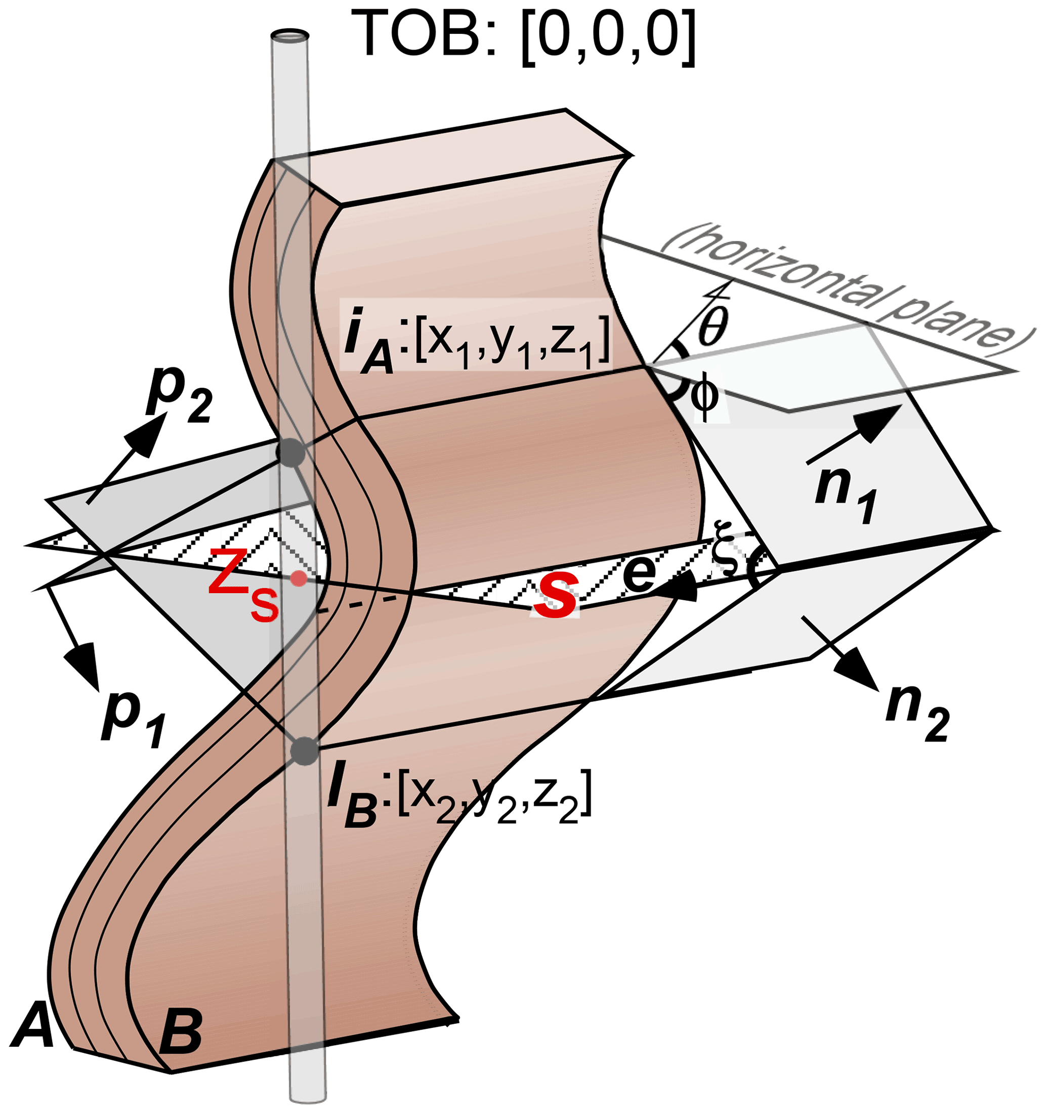
Figure 2Schematic illustration of a cylindrical concentric fold and a borehole. TOB is the top of the borehole. A and B represent folded bedding planes. n and p are the normal vectors of the bedding plane and inflexion surface, respectively. e is the direction vector of fold axis. S is the axial plane. iA, IB, and Zs are the intersection points of the borehole and A, B, and the axial plane. θ, ϕ, and ξ indicate strike, dip, and interlimb angle, respectively.
Note that the normal vector is a unit vector that does not include the spatial coordinates of the measured point. The direction vector of the fold axis e appears as the intersection of the following two planes:
The interlimb angle of a fold (ξ), the angle between the bedding planes, can be expressed as follows:
Thus, the fold and interlimb angles can be easily inferred by identifying the inflexion points on any bedding plane. The axial plane and its location can be calculated if the inflexion points are identified on the same bed. However, such cases can only occur when the axial plane is perpendicular to the borehole, and it is rarely possible to calculate the axial surface in a simple way. To identify an axial plane, we consider an inflexion surface p that is perpendicular to the stratum surface at the inflexion point and parallel to the fold axis (Fig. 2). The normal vector of plane p and the equation of the surface are expressed as follows:
Due to the assumption of concentric folding, the inflexion surface p is the plane that passes through the inflexion points on all bedding planes and not just on bedding planes A and B. The axial plane is the bisector plane of p1 and p2. Thus, the equation of the axial plane s is expressed as follows:
The strike (θ3) and dip angle (ϕ3) of the axial plane are as follows:
Note that there are two bisecting surfaces. One of these is the axial plane. As the axial plane passes between inflexion points, it is sufficient to confirm that the intersection point Zs of the drilled hole and the axial plane are included between iA and IB. If the borehole is considered to be vertical ( and at all times), then the coordinates of the intersection of the axial plane and borehole (z3) can be calculated as follows:
The distribution of folds along the borehole can be obtained by calculating the location of the axial planes in the borehole for each fold.
To check the feasibility of the proposed method, an artificial fold was created, and the fold parameters were calculated and compared to a conventional method. A schematic geological model with loose folds was used to illustrate the application of the method proposed in this study. The geological model, including folds, was created based on the arc method described by Busk (1929; Wojtal, 1988), for mapping cylindrical concentric folds, and extended to three dimensions. First, we draw several spherical shells, L, centred at an arbitrary point O in space. The folded stratum surface is obtained by calculating the tangent surfaces at each intersection of L and an arbitrary line l and projecting them onto a line segment that simulates a borehole (Fig. 3). The intersection of the outermost spherical shell and the inner spherical shell (L11 and L13 in Fig. 3) with l becomes the inflexion point of the fold. For the next deeper fold, the spherical shells and line are arbitrarily set and projected into the borehole in the same manner. To simulate the continuous development of folds, these two folds were set up to share an inflexion point (the layer enclosed by the square in Fig. 3).
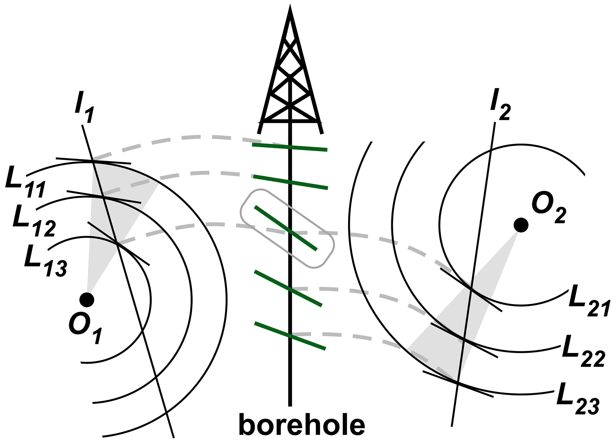
Figure 3Schematic diagram of the procedure for creating a simulated fold model. The grey hatch in the figure represents a fold created based on an arbitrary point O, and the green lines are the stratigraphic surface projected onto the borehole.
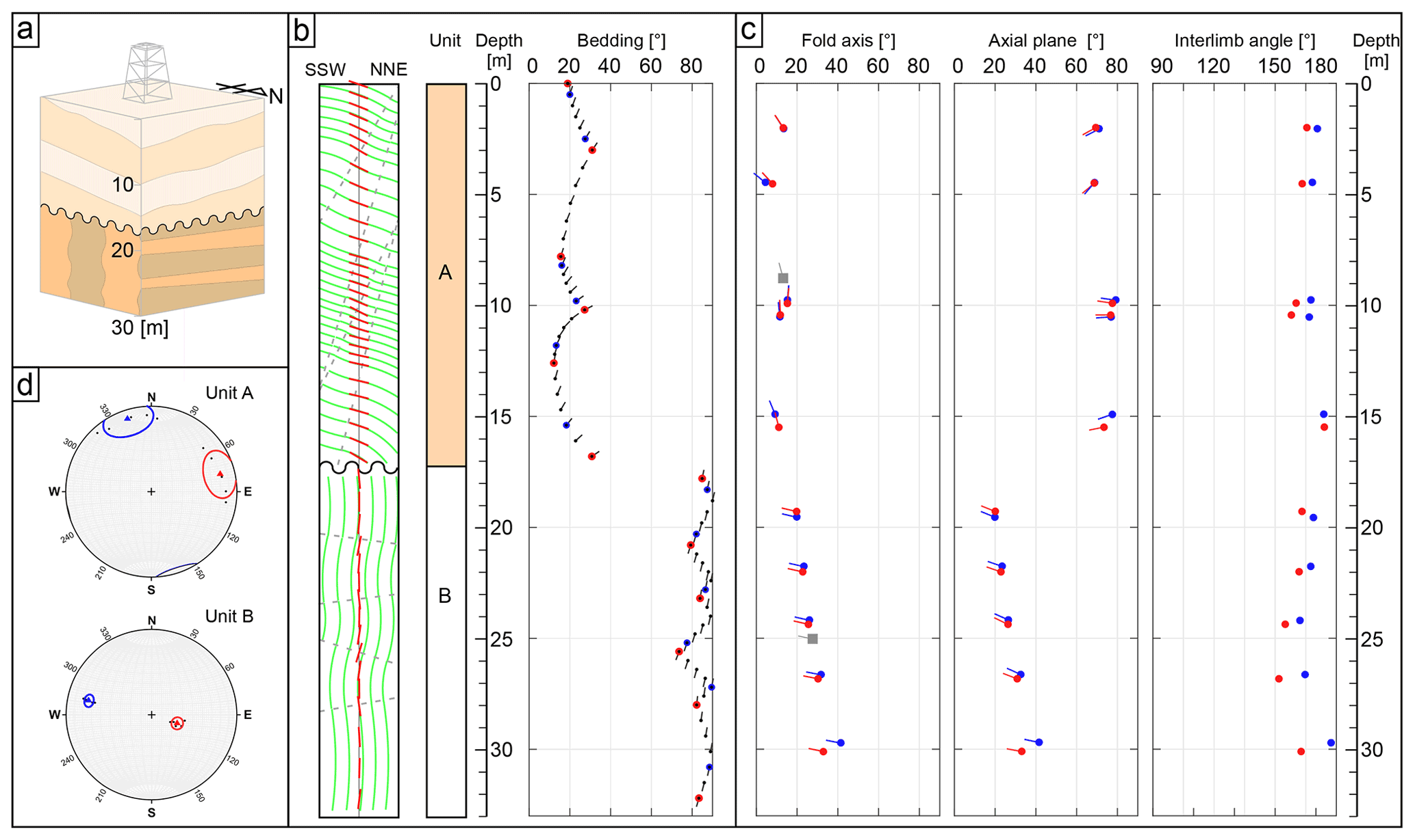
Figure 4Results of applying the proposed method to the simulated fold model. (a) Schematic image of the simulated fold model. (b) Cross section of the simulated fold model, structural units, and a tadpole plot of the orientation of bedding planes that would be interpreted if the simulated formation is drilled. Points identified as inflexion points are indicated by red/blue circles. (c) Fold axes, axial planes, and interlimb angles obtained by applying the proposed method. The grey squares represent the orientation of the fold axes calculated using the Bingham axial distribution for each unit. The difference between the red and blue circles is the same as the colour of the inflexion points used in the calculation. (d) Stereonet of calculated fold parameters. The mean direction (Fisher et al., 1987) of the poles of the axial planes is shown in red and that of the fold axis in blue, representing the direction of maximum principal stress and intermediate stress during fold formation, respectively. Curves of the same colour as the mean vector represent 95 % confidence cone for the mean direction (Fisher et al., 1987).
In this study, 10 folds were created to examine the proposed method. In total, seven spherical shells corresponding to the seven strata were utilized for each fold. There were two structural units with significantly different trends established for each of the five folds, and the fold structures were non-continuous between these units. Figure 4a and b display the stratigraphic model and the tadpole plot of the bedding strike and dip obtained from the interpretation of the borehole image logging. In Fig. 4b, the green line in the cross section indicates the bedding plane, and the grey dotted line and red points in the tadpole plot exhibit the inflexion plane and inflexion points of the folding strata, respectively. The fold axis is simply calculated by applying the Bingham axial distribution method (Fisher et al., 1987) to the unit-by-unit strike and dip data of this formation. The results of the general calculation, the azimuth, and plunge of the fold axis for units A and B were obtained to be 345, 13.3, and 282.1, 27.7, respectively.
The fold axis, axial plane, and interlimb angle were calculated for each fold according to its depth by applying the proposed method to the model data (red points in Fig. 4c). The axes calculated by the general Bingham axial distribution method are also plotted as grey rectangles in the plot of the fold axis in Fig. 4c. The proposed method provides considerable information on the fold components than the previous method. With the availability of axial planes, it is possible to estimate the stress direction in three dimensions (Fig. 4d). In addition, the amount of fold shortening can be determined from the interlimb angle. As each piece of information can be obtained continuously in the depth direction, it can also be used to detect the presence of local stress distribution or an overprinting fold by capturing changes in the axis or axial plane in a certain direction, as seen in unit B (Fig. 4d).
On the other hand, inflexion points do not always appear on the image log because of missing data or thick strata. For such cases, we also examined the way the estimated fold information would be affected by picking incorrect inflexion points. We performed calculations when the true inflexion point (red point) in Fig. 4b did not appear in the log, and the blue point was interpreted as the inflexion point. In this case, the shifting of an inflexion point causes a certain fold to contain a shortened section or to include strata of a different fold trend. The calculation results (blue points in Fig. 4c), however, exhibit no significant difference between the case where the wrong inflexion point is identified, and the case where the true inflexion point is selected. In particular, there is little change in the trend with depth or the value of the dip angle. However, it should be noted that the calculated depth of the folds may change, the interlimb angle can be overestimated (resulting in loose folds), and the observation error at this inflexion point may be difficult to estimate in practice. The values of the orientation of the simulated bedding planes and the evaluated fold parameters in the above calculations are provided in the Supplement.
The proposed method focuses only on the inflection points of the folds (maximum and minimum values in tadpole plots) and aims to mainly extract the fold parameters along the borehole. In this respect, it differs from the graphical representation of 2D/3D fold structures, including the Busk (1929) method, which uses continuous bedding data (e.g. Yamada et al., 2016). The advantage of our method is that, unlike previous methods aimed at reconstructing structures, it is simple and allows numerical data on continuous folds in the direction of the borehole to be calculated, even for small structures. The proposed method for deriving fold parameters assumes cylindrical concentric folds and can be applied to other cylindrical folds to some extent. In the case of parallel and symmetrical folds, the folding parameters can be calculated in the same way as for concentric folds, since the characteristics of the inflectional surfaces are the same as for concentric folds. In the case of a similar fold, the orientations of the fold and axial planes calculated by the same process would be equal to the actual fold parameters. The intersection of the axial plane and the borehole, corresponding to the calculated location of the fold, will be somewhat off, although it will be limited to between the inflexion point depths (see the Supplement). However, most folds in nature are cylindrical or conical folds, as pointed out by Wilson (1967). When this method is applied to conical folds, it results in the identification of meaningless axes. However, if the fold is symmetric, it is possible to evaluate a plausible axial plane. Other situations where this method is difficult to apply include those where the angle between the axial plane and the borehole is small, and those where the interlimb is nearly 0∘. This is because the variation in the bedding orientation due to folding is difficult to capture, and the frequency of crossing inflexion points may decrease. Very fine folds, such as those found in outcrops (e.g. Alexander and Watkinson, 1989) may be overlooked, or the heterogeneity of the stratum surface can be picked up in borehole images. In addition, errors can be introduced by incorrectly selecting inflection points (Fig. 4), and pseudo-folds can be identified due to the assumption that the strata are continuous. Caution should be exercised in attempting to estimate a wide range of precise fold structures using single borehole wall images. It may be necessary to identify several folds to focus on trends and perform statistical processing in these situations.
The proposed method will become even more effective for its use in detailed fold analysis by considering the seismic images and surrounding tectonics. Seismic imaging, however, may not be able to illustrate significant geological structures for the following reasons: lack of resolution, high dip angle of the bedding planes, and small differences in acoustic impedance (Serra, 2003). The proposed method using borehole and logging data will also be effective, especially in such cases, to clarify the invisible formation. The strength of this method is in the fact that it uses borehole images to quantitatively determine the location of the folded structures in the borehole. This can be utilized to create more realistic geological models, geological interpretation focusing on structural changes at depth, and structural geological interpretation, such as the estimation of present and past stress directions. Comparisons with other structural exploration methods, such as seismic reflection methods, and the use of data from multiple boreholes will enable the above strengths to be more robustly exploited.
The method described herein enables the determination of the azimuth and plunge of the fold axis, the strike and dip of the axial plane, the interlimb angle, and their depths from the bedding orientation acquired from the borehole image. To apply this method, we require marking the position of the inflexion point in the depth profile of the dip/strike of the bedding. It was confirmed that these fold parameters did not vary significantly, even when the inflexion points could not be reliably determined. This method was designed to be applied to cylindrical concentric folds, and it is also appropriate for the calculation of the axial plane orientation of symmetric folds. As it is difficult to limit the type of folds in borehole images, the method should be implemented with an understanding of the type of error that will occur if the actual formation is not a cylindrical fold. This method, which can obtain fold parameters continuously in the depth direction, will develop a geological interpretation using borehole image logs. If combined with other methods that can add information from a tadpole plot with regards to whether a fold is similar or not, then the result will be more advanced and user-friendly.
All data, including simulated dip and strike data used for fold calculations and the results of fold parameter evaluations, are shown in Sect. 3 and the Supplement.
The supplement related to this article is available online at: https://doi.org/10.5194/sd-31-85-2022-supplement.
YS and YH curated research data. YH and TH developed the model code and performed the simulations. YH prepared the paper with contributions from all co-authors.
The contact author has declared that neither they nor their co-authors have any competing interests.
Publisher’s note: Copernicus Publications remains neutral with regard to jurisdictional claims in published maps and institutional affiliations.
We are grateful to Yuzuru Yamamoto and Takamitsu Sugihara, for their helpful discussions. We would like to thank Editage for the English language editing. This work was partly supported by the Japan Society for the Promotion of Science KAKENHI (grant nos. JP21H05201, 20K14587, 19K21907, 19H02006, 19H00717, and JP16H06476) in the Scientific Research on Innovative Areas as part of the “Science of Slow Earthquakes” project.
This research has been supported by the Japan Society for the Promotion of Science (grant nos. JP21H05201, 20K14587, 19K21907, 19H02006, 19H00717, and JP16H06476).
This paper was edited by Ulrich Harms and reviewed by Maria Jose Jurado and one anonymous referee.
Alexander, J. I. D. and Watkinson, A. J.: Microfolding in the Permian Castile formation: An example of geometric systems in multilayer folding, Texas and New Mexico, Geol. Soc. Am. Bull., 101, 742–750, 1989.
Blake, K. and Davatzes, N. C.: Borehole image log and statistical analysis of FOH-3D, Fallon Naval Air Station, NV Proceedings Thirty-Seven Stanford University Geothermal Workshop, 30 January–1 February 2012, Stanford, California, USA, https://pangea.stanford.edu/ERE/db/IGAstandard/record_detail.php?id=8231 (last access: 30 May 2022), 2012.
Busk, H. G.: Earth flexures, Cambridge University Press, London, 106 pp., ISBN 9781107663190, 1929.
Crow, H. L. and Ladevèze, P.: Downhole geophysical data collected in 11 boreholes near St-Édouard-de-Lotbinière, Québec, Geological Survey of Canada, Open File 7768, 48 pp., https://doi.org/10.4095/297047, 2015.
Etchecopar, A. and Bonnetain, J. L.: Cross sections from Dipmeter Data 1, AAPG Bull., 76, 621–637, https://doi.org/10.1306/BDFF888A-1718-11D7-8645000102C1865D, 1992.
Etchecopar, A. and Dubas, M. O.: Methods for geological interpretation of dips, SPWLA, SPWLA-1992-J 33rd Annual Logging Symposium, 14–17 June 1992, Oklahoma City, Oklahoma, USA, https://onepetro.org/SPWLAALS/proceedings-abstract/SPWLA-1992/All-SPWLA-1992/SPWLA-1992-J/18977 (last access: 30 May 2022), 1992.
Fisher, N. I., Lewis, T. L., and Embleton, B. J.: Statistical Analysis of Spherical Data, Cambridge University Press, 329 pp., ISBN 9780511623059, 1987.
Goldberg, D.: The role of downhole measurements in marine geology and geophysics, Rev. Geophys., 35, 315–342, https://doi.org/10.1029/97RG00221, 1997.
Holdsworth, R. E.: The stereographic analysis of facing, J. Struct. Geol., 10, 219–223, 1988.
Ienaga, M., McNeill, L. C., Mikada, H., Saito, S., Goldberg, D., and Casey Moore, J.: Borehole image analysis of the Nankai Accretionary Wedge, ODP Leg. 196: Structural and stress studies, Tectonophysics, 426, 207–220, https://doi.org/10.1016/j.tecto.2006.02.018, 2006.
Lai, J., Wang, G., Wang, S., Cao, J., Li, M., Pang, X., Han, C., Fan, X., Yang, L., He, Z., and Qin, Z.: A review on the applications of image logs in structural analysis and sedimentary characterization, Mar. Petrol. Geol., 95, 139–166, https://doi.org/10.1016/j.marpetgeo.2018.04.020, 2018.
Mayer, J. J. and Albat, H. M.: An appraisal of the significance of small-scale fold structures in the contorted bed of the area of the Vredefort, S. Afr. J. Geol., 93, 311–317, 1990.
Moore, G. F., Kanagawa, K., Strasser, M., Dugan, B., Maeda, L., Toczko, S., and the IODP Expedition 338 Scientific Party: IODP Expedition 338: NanTroSEIZE Stage 3: NanTroSEIZE plate boundary deep riser 2, Sci. Dril., 17, 1–12, https://doi.org/10.5194/sd-17-1-2014, 2014.
Prensky, S. E.: Advances in borehole imaging technology and applications, Geological Society, London, Special Publications, edited by: Lovell, M. A., Williamson, G., and Harvey, P. K., Geological Society, London, 159, 1–43, https://doi.org/10.1144/GSL.SP.1999.159.01.01, 1999.
Ramsay, J. G. and Huber, M. I.: The techniques of modern structural geology, in: Folds and Fractures, vol. 2, Academic Press, London, ISBN 0125769024, 1987.
Scott, R. J. and Selley, D.: Measurement of fold axes in drill core, J. Struc. Geol., 26, 637–642, https://doi.org/10.1016/j.jsg.2003.08.016, 2004.
Serra, O. L.: Well Logging and Geology, Editions Serralog, Mery Corbon, France, ISBN 9782951561618, 2003.
Tobin, H., Hirose, T., Saffer, D., Toczko, S., Maeda, L., Kubo, Y., Boston, B., Broderick, A., Brown, K., Crespo-Blanc, A., Even, E., Fuchida, S., Fukuchi, R., Hammerschmidt, S., Henry, P., Josh, M., Jurado, M. J., Kitajima, H., Kitamura, M., Maia, A., Otsubo, M., Sample, J., Schleicher, A., Sone, H., Song, C., Valdez, R., Yamamoto, Y., Yang, K., Sanada, Y., Kido, Y., and Hamada, Y.: Site C0002, in: Integrated Ocean Drilling Program. Proceedings IODP, 348, edited by: Tobin, H., Hirose, T., Saffer, D., Toczko, S., Maeda, L., Kubo, Y., and the Expedition 348 Scientists, College Station, TX, https://doi.org/10.2204/iodp.proc.348.103.2015, 2015.
Vickerman, K. and Spratt, D.: Measuring minor structures in borehole image logs, CSPG CSEG CWLS Convention, 9–11 May 2011, Calgary, Alberta, Canada, https://cseg.ca/resources/abstracts/2011-conference-abstracts-m-to-z (last access: 30 May 2022), 2011.
Wilson, G.: The geometry of cylindrical and conical folds, P. Geologist. Assoc., 78, 179–209, https://doi.org/10.1016/S0016-7878(67)80043-9, 1967.
Wojtal, S.: Chapter 13 Objective methods for constructing profiles and block diagrams of folds, in: Basic Methods of Structural Geology, edited by: Marshak, S. and Mitra, G., Prentice-Hall, Englewood Cliffs, NJ, USA, 269–302, ISBN 0130652105, 1988.
Yamada, T., Le Nir, I., Moscardi, E., and Etchecopar, A.: A new parallel fold construction method from borehole dip for structural delineation, AAPG Annual Convention and Exhibition, 19–22 June 2016, Calgary, Alberta, Canada, https://www.searchanddiscovery.com/pdfz/documents/2016/41969yamada/ndx_yamada.pdf.html (last access: 30 May 2022), 2016.
Zemanek, J., Caldwell, R. L., Glenn, E. E., Jr Holcomb, S. V., Nortom, L. F., and Siraus, A. D. J.: The Borehole Televiewer – A New Logging Concept for Fracture Location and Other Types of Borehole Inspection, J. Petrol. Technol., 264, 762–774, https://doi.org/10.2118/2402-pa, 1969.