A strainmeter array as the fulcrum of novel observatory sites along the Alto Tiberina Near Fault Observatory

Fault slip is a complex natural phenomenon involving multiple spatiotemporal scales from seconds to days to weeks. To understand the physical and chemical processes responsible for the full fault slip spectrum, a multidisciplinary approach is highly recommended. The Near Fault Observatories (NFOs) aim at providing high-precision and spatiotemporally dense multidisciplinary near-fault data, enabling the generation of new original observations and innovative scientific products.

The Alto Tiberina Near Fault Observatory is a permanent monitoring infrastructure established around the Alto Tiberina fault (ATF), a 60 km long low-angle normal fault (mean dip 20°), located along a sector of the Northern Apennines (central Italy) undergoing an extension at a rate of about 3 mm yr⁻¹. The presence of repeating earthquakes on the ATF and a steep gradient in crustal velocities measured across the ATF by GNSS stations suggest large and deep (5–12 km) portions of the ATF undergoing aseismic creep.

Both laboratory and theoretical studies indicate that any given patch of a fault can creep, nucleate slow earthquakes, and host large earthquakes, as also documented in nature for certain ruptures (e.g., Iquique in 2014, Tōhoku in 2011, and Parkfield in 2004). Nonetheless, how a fault patch switches from one mode of slip to another, as well as the interaction between creep, slow slip, and regular earthquakes, is still poorly documented by near-field observation.

With the strainmeter array along the Alto Tiberina fault system (STAR) project, we build a series of six geophysical observatory sites consisting of 80–160 m deep vertical boreholes instrumented with strainmeters and seismometers as well as meteorological and GNSS antennas and additional seismometers at the surface.

By covering the portions of the ATF that exhibits repeated earthquakes at shallow depth (above 4 km) with these new observatory sites, we aim to collect unique open-access data to answer fundamental questions about the relationship between creep, slow slip, dynamic earthquake rupture, and tectonic faulting.

1 Introduction

1.1 TABOO NFO – the infrastructure

The Alto Tiberina Near Fault Observatory (TABOO NFO; Chiaraluce et al., 2014; Caracausi et al., 2023) is a state-of-the-art geophysical network, managed by the Istituto Nazionale di Geofisica e Vulcanologia (INGV), composed of modern seismological, geodetic, and geochemical stations placed along an extending sector of the Northern Apennines of Italy containing fault systems recently activated by a series of moderate magnitude earthquakes (5 < M_w < 6.5; Fig. 1).

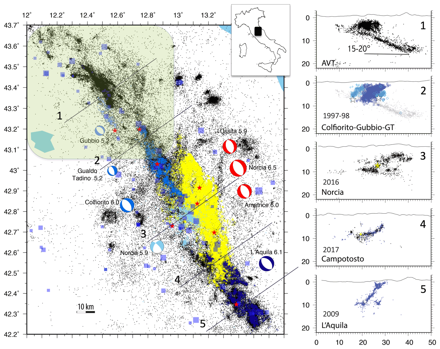
Figure 1 Map of the sector of the Northern Apennines, currently extending at about 3 mm yr⁻¹ in the NE-trending direction. The southern portion was hit both recently and in historical times (light-blue squares represent historical earthquakes from CPTI15; Rovida et al., 2022) by a series of moderate magnitude earthquakes. From south to north, the seismic sequences are L'Aquila, 2009 (dark blue); the most recent 2016–2017 central Italy sequence (yellow); Norcia, 1979 (celestine); Colfiorito, 1997, and Gualdo Tadino, 1998 (blue); and Gubbio, 1984 (light blue). These sequences activated a 150 km long extensional fault system over the last 25 years. The TABOO study area is located north in the region highlighted in green where, differently from the southern area, we have no large historical earthquakes and a continuous release of microearthquakes with no events larger than M 4, occurring along an east-dipping fault at a very low angle (15–20°). This large and misoriented fault continuously generates microearthquakes along a structure dipping in the opposite direction relative to all the other segments activated during the large seismic sequences (see cross-sections).

The fault system monitored by TABOO NFO is dominated at depth by the Alto Tiberina fault (ATF), an east-dipping low-angle normal fault (mean dip 20°; see the topmost section in Fig. 1), which, if activated along its entire surface (60 × 40 km, reaching 15 km of depth), could generate an earthquake of magnitude up to 7. It is worth noting that such an event is not present in the Italian catalog of historical earthquakes for that portion of the Northern Apennines, and this range of magnitude can be considered complete for the past 900 years (Visini et al., 2022).

Along the ATF, in the last 40 years, in terms of instrumental earthquakes, we have only recorded events smaller than M_w 3, occurring at a high and almost continuous rate (Chiaraluce et al., 2007; Valoroso et al., 2017; Cattaneo et al., 2017; Vuan et al., 2020), whilst on its hanging wall, along shallower and minor syn- and antithetic splays dipping at higher angle (up to 45–60°), we detect seismic sequences with mainshocks reaching up to M_w 4.5.

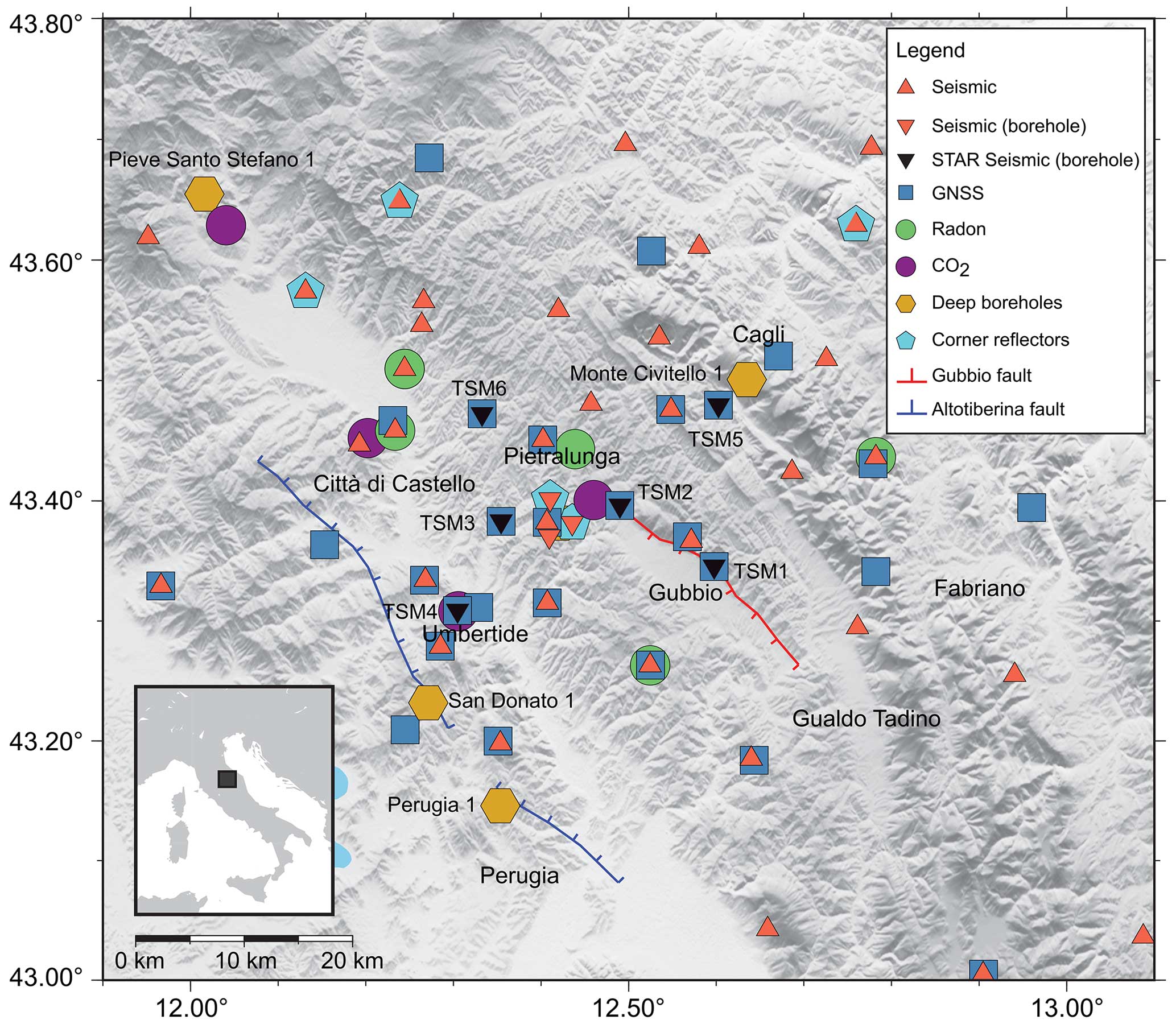
Figure 2 Map of TABOO NFO infrastructure and station distribution with respect to the ATF (blue line) and Gubbio fault (red line). Orange triangles are seismic stations deployed at the surface and within shallow boreholes. Blue squares and turquoise pentagons are GNSS stations and corner reflectors, respectively. Green and purple circles are, respectively, Rn and CO₂ monitoring sites, while the kilometer-deep boreholes are reported with yellow hexagons. The six observatory sites (STAR project, TSM1 to TSM6) are instead represented as black upside-down triangles. Figure generated with GMT (Generic Mapping Tools).

With a mean inter-distance of about 8 km between the sites (Fig. 2), starting from 2010, TABOO's multidisciplinary sensors deployed both at the surface and within shallow boreholes (< 250 m) collect near-fault data to capture a very broad range of signatures related to tectonic deformation processes. All TABOO NFO's seismic, geodetic, and geochemical sensors record and transmit in real time, via dedicated Wi-Fi technology. Seismic and geodetic raw data are discoverable and accessible in standard formats on dedicated repositories (e.g., https://eida.ingv.it/it/, last access: 17 June 2024​​​​​​​, and https://gnssdata-epos.oca.eu/#/site, last access: 17 June 2024), while meteorological and geochemical data (Rn, CO₂) and all the derived multidisciplinary scientific products are discoverable on open-access thematic portals and accessible via dedicated web services on thematic portals (http://fridge.ingv.it, last access: 17 June 2024, and https://www.epos-eu.org/dataportal, last access: 17 June 2024).

1.2 ATF system and STAR project

Consistent with the existing TABOO NFO geodetic data (Vadacca et al., 2016), the interpretation of the seismic reflection profiles provided by the CROP03-NVR survey (Crosta Profonda Project Near Vertical Reflection; Pialli et al., 1998; Pauselli et al., 2006) shows that a significant amount of Neogene–Quaternary extension within the Northern Apennines brittle upper crust is accommodated by a system of east-dipping LANFs (low-angle normal fault) with associated high-angle antithetic structures. The ATF is the most easterly and most recently formed among the LANFs contributing to the distributed faulting responsible for a significant portion of the documented tectonic extension within the Apennines belt. A long-term aseismic slip rate of 1.7 mm yr⁻¹ is reported by geodetic data, contributing to the total amount of 3 mm yr⁻¹ of extension ongoing in this sector of the Apennines (Anderlini et al., 2016).

Existing data from TABOO NFO support the hypothesis that portions of the ATF creep aseismically.

Seismicity data reveal microseismic release at a consistently high rate occurring along the ATF plane, including repeating earthquakes (REs; Valoroso et al., 2017; Vuan et al., 2020). A steep gradient in crustal velocities measured by GNSS (Vadacca et al., 2016) and interpreted as the signature of creeping occurring below 5 km of depth along the ATF plane and transient motion detected by GPS arrays lasting for a few months and coinciding with seismic swarms (Gualandi et al., 2017).

Recent studies document that any given patch of a fault can creep, nucleate slow earthquakes, and host large earthquakes (e.g., Iquique earthquake, Ruiz et al., 2014; Tōhoku earthquake, Kato et al., 2012; and Parkfield earthquake, Veedu and Barbot, 2016). The hypothesis that a fault patch would switch from one sliding mode to another is contrary to ordinary theory. Thus, these observations are forcing a revolution in our way of thinking about how faults accommodate slip. However, the interaction between creep, slow, and regular earthquakes is still poorly documented by observation.

With STAR (strainmeter array along the Alto Tiberina fault system; https://www.icdp-online.org/projects/by-continent/europe/star-italy, last access: 17 June 2024), a project co-founded by ICDP, NSF-US, and INGV, we aim to collect the data required to address these topics. By installing a set of six strainmeters that will be part of the existing TABOO NFO infrastructure, STAR will provide unique open-access data to answer fundamental questions about the relationship between creep, slow slip, dynamic earthquake rupture, and tectonic faulting. The strainmeter array (STAR) instruments can resolve the full horizontal strain tensor for deformation on the order of the nano-strain, with temporal sampling (> 20 Hz) shorter than timescales typically explored by GNSS. TABOO NFO instrumentation will thus resolve the spatiotemporal pattern of slip on the ATF with sufficient resolution on timescales (minutes to days to months) that appear to characterize transient aseismic slip worldwide. Our goal is to obtain high-resolution observations of deformation processes to better understand the physical processes that enable both seismic and aseismic slip on a single fault patch, with potentially revolutionary implications for seismic hazard and risk assessment. Moreover, given the very local scale of our observatory network, we may bridge the gap between laboratory and natural-scale observations. Each observatory site is also equipped with surface GNSS, meteorological instruments, and additional seismic sensors. Moreover, the two deepest boreholes host fiber-optic cables for temperature and strain. Four out of six holes host pressure transducers to correct the strainmeter data.

An additional motivation for STAR is the presence in the ATF system volume of deep fluid circulation. The observed flux of natural CO₂ in central Italy, where the ATF is located, is comparable to that from worldwide active volcanic systems, making the ATF an ideal site for studying the relationship between fluids that move from the whole crust towards the atmosphere (e.g., Italiano et al., 2009), seismicity pattern, strain, and faulting. The existence of fluid transport processes is supported, as already highlighted, by the evidence that within deep boreholes drilled in this area and located in the ATF footwall (Pieve Santo Stefano 1 and San Donato 1; Fig. 2), fluid overpressure (CO₂) at about 85 % of lithostatic load has been encountered. In addition, the isotopic signature of fluids emitted in many local springs with gaseous emissions indicates that the whole area is affected by an extremely large flux of CO₂ from a deep source (e.g., Rogie et al., 2000; Chiodini et al., 2004; Italiano et al., 2009). The over-pressurization from below by deep derived CO₂ is proposed as being one of the primary triggering mechanisms of the Apennines earthquakes (Chiodini et al., 2004). That is why TABOO hosts four Rn and four CO₂ geochemical stations (Caracausi et al., 2023) that measure the output of these volatiles at high frequency and monitoring the high flux of CO₂ gas emissions at low frequency in order to investigate the sources of fluids (mantle vs. crust) and how secondary processes (e.g., rock–water–gas interaction) during the transport and storage of the fluids within the crust can modify the chemistry of the fluids (Ventura Bordenca, 2020).

Thus, with the new observatory sites, TABOO NFO will acquire novel high-precision data, allowing for a quantitative characterization of ATF creep (∼ 1 mm over < 1 km), enhanced monitoring of microseismicity (below M_c 0.5), and investigation of possible correlation between degassing (CO₂, Rn) measurements and subsurface deformation. Such unique near-fault data may illuminate the spatiotemporal characteristics of creep on the ATF, permitting detailed analysis of potential stress interactions with the overlying hanging wall faults known to host larger earthquakes. The interdisciplinary observations are needed to address key questions of global importance in the seismic hazards and risk assessment community about the physics that allows for both seismic and aseismic slip on a single fault patch.

After presenting the field campaigns, we give an overview of the new strainmeter and seismometer data, showing how they enable us to detect dynamic and static strain otherwise missed by other existing in situ instruments.

2 STAR field campaign

2.1 Site selection

The six boreholes of the STAR project (Fig. 2) were drilled in northern Umbria, in an area between the High Tiber Valley, bordered by the east-dipping ATF, and the western flank of the main ridge of the Umbria-Marche Apennines, a NE-verging, arc-shaped foreland fold-and-thrust belt, representing the eastern part of the Northern Apennines of Italy (Fig. 3a; Barchi, 2010).

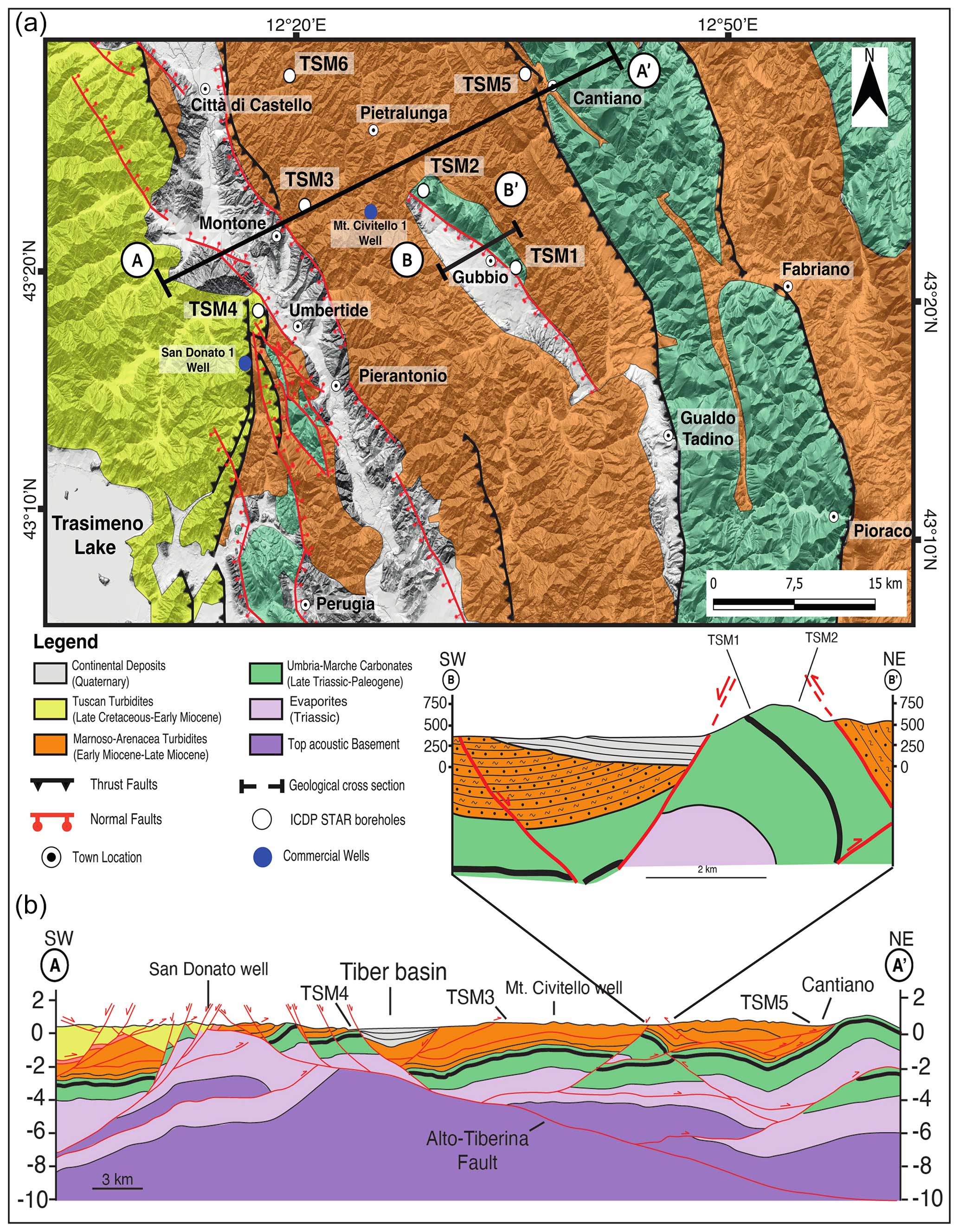
Figure 3 Schematic geological map (a) and geological sections (b) across the TABOO area. The map shows the locations of the six STAR boreholes (white circles) and of the two deep boreholes (San Donato 1 and Mt. Civitello 1, blue circles). The geological cross-sections A–A' and B–B' illustrate the geometry at depth of the major, contractional and extensional, tectonic structures affecting the study area, relative to the position of the STAR boreholes. The deep structures of section A–A' have been constrained through the interpretation of a set of seismic reflection profiles: the black layer within the Umbria-Marche carbonates represents the Marne a Fucoidi formation, which corresponds to a major seismic marker. Figure modified from Mirabella et al. (2011).

The NNW–SSE-trending compressional structures (folds and thrusts) of this region were formed in the Late Miocene (Tortonian–Messinian age) and involve a Jurassic–Paleogene carbonate succession (Umbria-Marche succession; e.g., Cresta et al., 1989), deposited on the southern (African) margin of the Western Tethys, overlain by a thick succession of Neogene turbidites, marls, and sandstones, deposed in the foreland ramp and in the foredeep of the syntectonic, foreland basin of the Northern Apennines. The compressional structures are cut and displaced by later (Late Pliocene–Quaternary) normal faults, responsible for the present-day seismicity of the region, whose study and characterization are the main objective of the STAR project.

In the central part of the area, the Mesozoic carbonates are exposed at the core of the prominent Gubbio anticline, whose back limb is downthrown by the SW-dipping Gubbio fault, representing the most important antithetic splay of the ATF (e.g., Mirabella et al., 2004, 2011).

The stratigraphy of the six boreholes and their location with respect to the main geological structures are summarized in Table 1 and illustrated in the geological section of Fig. 3b.

Table 1 List of key depths for the six boreholes.

Two sites (TSM1 and TSM2) were drilled across the late Mesozoic–early Tertiary carbonates, cropping out along the crest of the Gubbio anticline, which represents the maximum structural culmination of the study area. All the other wells were all drilled in the Neogene marls and sandstones: TSM4 is located at the ATF footwall block, west of the Tiber Valley; TSM2 and TSM6 were drilled in the ATF hanging wall block, in the northern part of the study area; and TSM5 was drilled in the northeastern part, close to the western flank of the Umbria-Marche ridge (Fig. 3b).

Within the ATF seismicity, we observed that REs occur within the geodetically recognized creeping portions of the ATF, around an apparent locked asperity located in the northern portion of the fault placed between the settlements of Città di Castello and Gubbio (Valoroso et al., 2017; Anderlini et al., 2016). The rate of occurrence of REs has also been observed as synchronous with hanging wall swarms, suggesting that creeping may guide strain partitioning in the ATF system (Vuan et al., 2020). In detail, the seismic moment released from the ATF seismicity only accounts for about 30 % of the observed geodetic deformation, confirming the need for aseismic deformation (Gualandi et al., 2017). This implies that the ATF seismicity pattern is consistent with a mixed-mode (seismic and aseismic) slip behavior (as defined by Avouac, 2015). As pointed out above, the occurrence of slow and fast earthquakes on the same fault patch has revolutionized our thinking about how faults accommodate slip. However, the interaction between creep, slow, and regular earthquakes is still elusive, primarily due to the dearth of high-resolution observations across the spectrum of slip phenomena. In this context, the ATF is a particularly fruitful location for such an investigation at the local scale, as demonstrated in Gualandi et al. (2017), where the dense GNSS network allowed for the detection of a very small amplitude transient deformation signal, correlated in both space and time with an intense seismic swarm (maximum M_w 3.7) that occurred in the ATF hanging wall in 2013 (Vuan et al., 2020). Thus, the northern portion of the ATF that hosted the aseismic deformation, located primarily in the footwall of the antithetic (SW-dipping) Gubbio fault (Fig. 2), was identified as a STAR target zone for drilling and instrument deployment.

2.2 Drilling operations

We drilled the six 80–160 m deep boreholes surrounding the creeping portion of the ATF (named TABOO borehole strainmeter, acronym TSM1–6; see locations in Fig. 2), to deploy Gladwin Tensor strainmeters and short-period seismometers, in a two-step fieldwork campaign: during the fall of 2021 and spring of 2022.

Boreholes were drilled using a Casagrande C8 rig using mud rotary drilling. Mud was made using a polymer drilling fluid. The preferred method of drilling a strainmeter borehole is to use an air hammer for the cased section of the borehole and an air rotary for the open section of the borehole. Traditional bentonite mud can be difficult to clean out of the borehole and can leave a thin layer on the walls of the borehole, which can prevent the strainmeter from properly coupling with the host rock. Using the polymer drilling fluid allowed for a smaller drill rig while enabling complete flushing of the borehole.

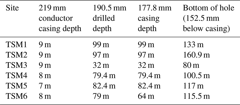
Boreholes are drilled in two phases. Phase 1 consists of drilling to 7–9 m and setting 219 mm conductor casing to prevent loose surface material from falling into the borehole. After the conductor casing is set, a 190.5 mm section is drilled to a depth where the rock appears to be stable (32–99 m). After reaching our casing target depth, the drill rod is removed, and 177.8 mm steel casing is lowered into the borehole. Before casing, the inclination of the borehole was checked using an EZDip inclinometer, with a goal of maintaining no more than 5° vertical deviation. The casing protects the borehole from collapsing and is critical for the installation of the strainmeter. After the casing is installed, the anulus was cemented using Portland cement. After the downhole work is complete, the casing is used as a stable GNSS monument.

Phase 2 of the drilling uses a 152.5 mm tricone drill bit to drill down to the installation zone. While the boreholes are being drilled, the operation is closely monitored. We look for excessive vibration, changes in drilling speed, and water production. These can indicate fractures or changes in lithology. We also collected cutting samples every 9 m. Once we had passed through several sections of what appears to be consistent material (smooth drilling and lack of water production), we stopped drilling and prepared to log the hole. Before logging, the borehole is flushed with clean water while moving the drill rod up and down. Water is sampled until polymer is no longer be detected. After the borehole was cleaned, we ran geophysical logging gear in the open borehole.

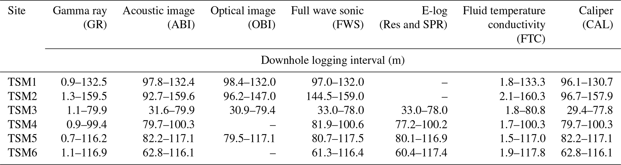
Table 2 Depth interval recorded by downhole logging sondes for each STAR borehole.

2.3 Downhole logging

Upon completion of the drilling operations, a suite of downhole logging measurements was performed in each borehole. The main purpose of these acquisitions was to select the most ideal section of rock formation to deploy at depth seismometers and strainmeters. The selected interval had to be as stable as possible with unfractured, competent rocks and with a very smooth borehole wall for coupling between instruments and rock formation. Thus, it was crucial to detect fractures/faults and weak zones intersecting the boreholes as well as their spatial distribution, characteristics, and connection with the geological structures mapped on the surface. Therefore, knowledge of petrophysical properties of drilled rock formation (i.e., Rider and Kennedy, 2011; Pierdominici and Kück, 2021) became key parameters for deep subsurface characterization, especially because no core material was available for further and more detailed geomechanical and structural analyses in laboratory.

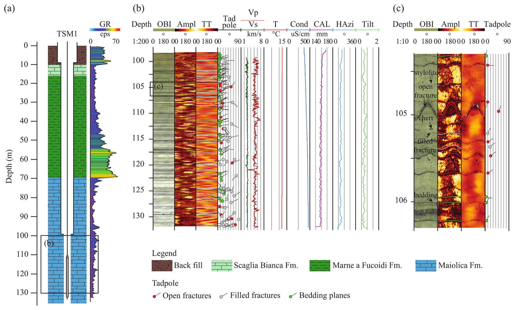
Figure 4 Downhole logging measurements executed in the borehole TSM1. (a) Lithological column with associated GR log acquired in both CH and OH. The GR shows a low signal in the carbonate rock (Maiolica formation) and higher values at the Marne a Fucoidi formation, especially between 60 and 70 m, where the GR reaches the highest values (around 60–70 cps) due to the higher clay contribution. (b) Geophysical logging measurements only in the OH: optical imager (OBI); borehole televiewer with amplitude and travel time images (Ampl and TT, respectively); Vp and Vs obtained from the analysis of the FWS, fluid temperature, and conductivity (T and Cond, respectively); and borehole geometry that includes the caliper (CAL) of the borehole calculated from TT, the hole azimuth (HAzi), and tilt from the three-arm caliper sonde. (c) An enlargement showing the geological structures identified on the borehole images. The tadpoles display their dip (colored dot) and dip azimuth (black tail).

Downhole logging measurements were acquired in fall 2021 and summer 2022 by a logging contractor (GEOLOGIN). All six shallow boreholes were logged by slim-hole sondes (Table 2), and the following downhole measurements only cover the open hole (OH; uncased): acoustic televiewer (ABI), optical borehole imager (OBI), full waveform sonic (FWS), E-log (resistivity, Res, and single-point resistance, SPR), fluid temperature conductivity (FTC), three-arm caliper (CAL), and total gamma ray (GR). The latter also ran in the cased hole (CH; Fig. 4). All logging measurements were depth-matched using the gamma ray as the reference logging present in all sondes.

Table 3 Geophysical properties of the rocks.​​​​​​​

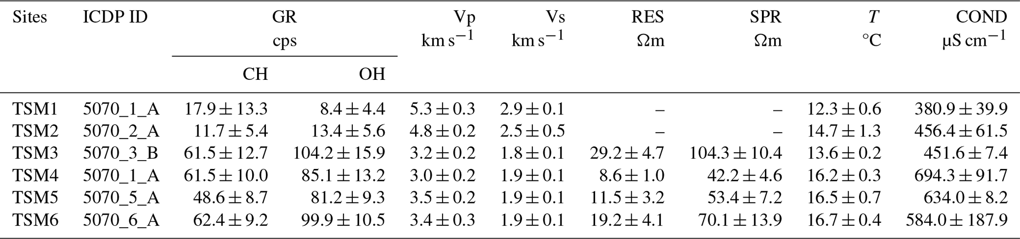
Within this paper, a brief and preliminary analysis of the downhole logging data is presented (Table 3), which will be the main focus of a separate contribution. Downhole logging in the OH carbonate units of boreholes TSM1 (Fig. 4b) and TSM2 (Maiolica and Scaglia Rossa formations) shows no significance in the gamma ray (values less than 15 cps). P- and S-wave velocities have mean values of 5.3 and 2.9 km s⁻¹, respectively, for the Maiolica formation (TSM1) and 4.8 and 2.5 km s⁻¹ for the Scaglia Rossa formation (TSM2). E-log has been not executed due to time constraints. In the sandstone–marly units (Marnoso-Arenacea formation), encountered in three boreholes (TSM3, 4, and 6), the gamma ray measurements provide higher values (about 80–100 cps), which are mainly correlated to marly intervals. In these three boreholes, P-wave velocities are similar, with values between 3.0 and 3.4 km s⁻¹, as are the S-wave velocities, which show constant values of about 1.9 km s⁻¹. E-log shows values less than 20 Ωm (Res) and 80 Ωm (SPR), with the exception of the TSM3 borehole, where a very hard and competent interval was encountered. In TSM5, the hemipelagic marls of the Schlier formation are characterized by a high gamma ray (mean value of 80 cps), by an average P- S wave velocity of about 3.5 and 1.9 km s⁻¹, and by low Res and SPR values. All six boreholes show fluid temperatures (T) between 12 and 10 °C. The fluid conductivity log (COND) has revealed values between 380 µS cm⁻¹ in the carbonate formations of TSM1 and 694 µS cm⁻¹ in the Marnoso-Arenacea formation of TSM4. The high value of COND recorded in TSM4 was ascribed to the proximity of a local spring (Fig. 4b, Table 3),

Table 4 Structural analysis from OBI and ABI image logs.​​​​​​​

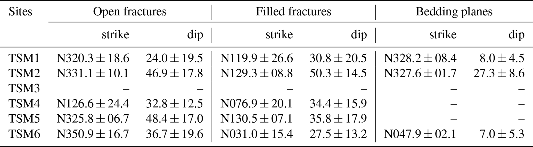
The televiewer and optical imager tools have delivered high-resolution images of the borehole wall. OBI was not performed in TSM4 and TSM6 boreholes. The televiewer sonde provides two 360° color-coded unwrapped images reflecting the roughness and shape of the borehole wall and its acoustic properties (Zemanek et al., 1969; Pierdominici and Kück, 2021). The analysis and evaluation of the OBI and ABI images allowed us to detect orientation and geometry of structures such as open or filled fractures and bedding planes but also additional geological features such as stylolites and cherts (Fig. 4c). Open and filled fractures were distinguished using purely OBI images, except for TSM4 and TSM6. For these two boreholes, the distinction between open and filled fractures was based on comparison of AMPL and TT images. Well-developed fractures visible in both images were classified as open, whereas those visible only in the AMPLs were defined as filled. Both fractures have on average a higher dip angle (Table 4) with a mean orientation of around NE–SW, while the bedding planes show a generally low dip angle and similar orientation.

The logging evaluation enabled the identification of intervals at depth not affected by fractures or weak zones that could affect the deployment of the instruments but especially the acquisition of seismic and deformation data.

2.4 Instrumenting

The primary STAR instrument is the Gladwin Tensor Strainmeter (GTSM). This instrument uses a capacitance bridge as a strain gauge to measure changes in length across a sensing volume. There are four horizontal strain gauges. The upper three gauges are oriented 120° from each other. The last gauge is 90° from the second gauge and 30° from the other two. This provides redundancy if a gauge fails. For proper coupling, the GTSM needs to be installed in competent rock without fractures and below any active aquifers. Once the suitable installation zone is selected based on the logging analysis, the borehole is prepared for installation. If the installation zone is more than a meter above the bottom of the borehole, it has to be lifted with Portland cement. If it is less than a meter above the bottom, gravel is used.

To properly couple the GTSM to the host rock, we used a cement able to expand. The preferred grout is BASF MasterFlow 1206 expansive grout (0 %–0.2 % expansion). The grout is mixed in a standard mortar mixer until completely hydrated with no lumps (20 s flow cone test). The grout is transferred to a dump baler. This is a 10.15 cm ID aluminum tube (9–12.5 m depending on rig tower height) with a valve on the bottom. The valve is opened when the baler hits the bottom of the borehole. The grout is released with minimum mixing with the fluids in the borehole. After the baler is removed from the borehole, the GTSM is lowered inside the hole using the same cable that carries the signal. Once the GTSM is lowered to the installation zone, its cable is tied off to the wellhead, and the installation equipment is cleaned up. No downhole work is done for the next 24 h to allow the grout to set.

The secondary instrument installed in the borehole is a three-component 2 Hz seismometer (see installation interval in Fig. 5), lowered on 50 mm PVC pipe. A section of slotted PVC is placed above the seismometer to sample an aquifer that is located using the geophysical logging data, usually 9–15 m above the seismometer. The seismometer is lowered until it reaches the top of the strainmeter grout. It is then pulled up by 1 m and finally cemented using the PVC pipe. The amount of cement is calculated to come up to the screen. The PVC is flushed with water to clear out the screen. TSM1 and TSM2 also have a loop of fiber-optic cable attached to the PVC pipe. Cement is allowed to cure until the next day. The final borehole work involves placing a sand pack around the screened section and a bentonite seal above the sand. After the bentonite hydrates, the hole is cemented up to the surface.

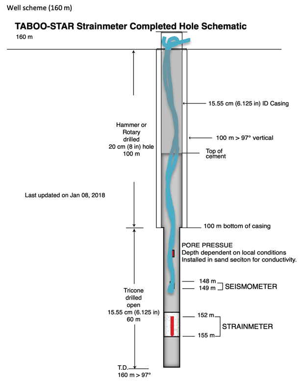
Figure 5 Schematic of the hole showing the strainmeter deployed in the deepest portion of the hole with the seismometer on top (see on the right side for details). The schematic also reports the adopted drilling techniques (see left side for details). The curved blue line represents the fiber-optic cable deployed only in the two deepest holes (see text for details).

The top of the borehole is completed with an adapter and GNSS antenna. After several weeks to months, the water level is measured in the PVC tube. A pressure sensor is lowered in the PVC 3–4 m below the water level. Surface sensors include rain and barometric pressure sensors and a seismometer.

In Table 5 we report the key depths of the strainmeters and seismometers at installation.

Table 5 Instruments' depths of deployment.

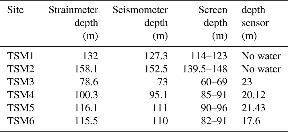
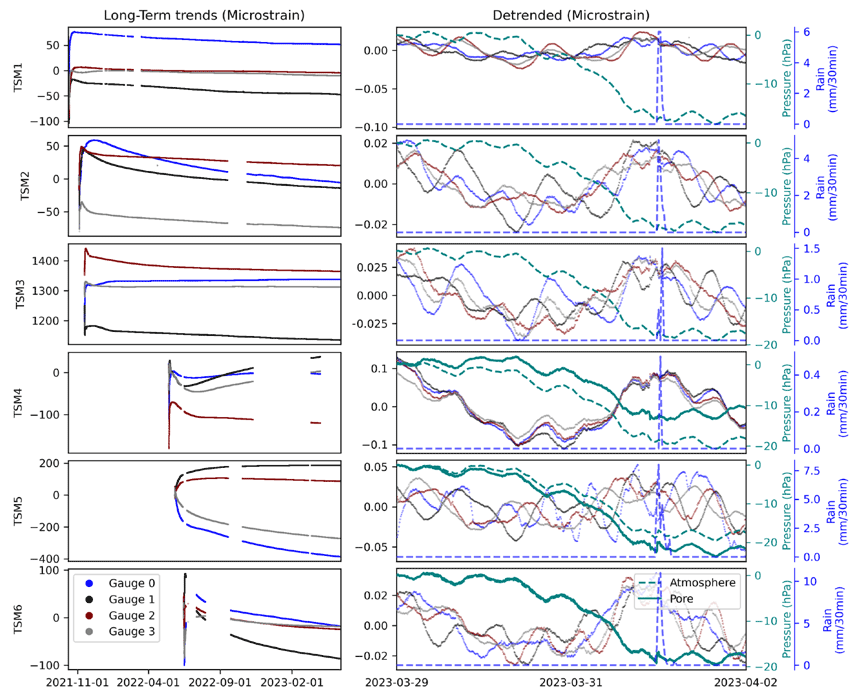
Figure 6 Demonstration of gauge strains for all STAR instruments. Plots on the left show the transition from initial grout curing following installation to long-term borehole relaxation. Plots on the right show the linearly detrended gauge strains, which are dominated by changes in atmospheric pressure changes and tidal strains. Pressure data from surface sensors and pore pressure sensors (TSM4, 5, and 6 because TSM3 was not recording pore pressure data at that time) are plotted on a separate y axis for comparison. All raw gauge data have been converted to units of linearized strain and plotted with different colors according to the figure legend shown in the bottom left. The pore pressure and barometric pressure data are plotted as solid and dashed teal lines, respectively. All data have had the first value of the time series subtracted. Raw strain records and pressure data are downloaded from EarthScope.

3 Data acquisition

3.1 Strainmeters

Currently, about a year after installation, all strainmeters demonstrate signs of proper functionality. Following installation, initial grout curing transitions toward long-term borehole “relaxation”, which typically manifests as a logarithmically decaying areal compression that persists through the lifetime of the station (Gladwin et al., 1987; Fig. 6). On the timescale of hours to days, the strainmeters respond to earth body tides and ocean loads, as well as atmospheric pressure changes, rainfall or groundwater flow (Fig. 6). The instruments likewise demonstrate superb capability for detecting high-rate dynamic strains, as depicted in Fig. 7 at TSM3 for the Umbertide M_w 4.3 earthquake ∼ 10 km away.

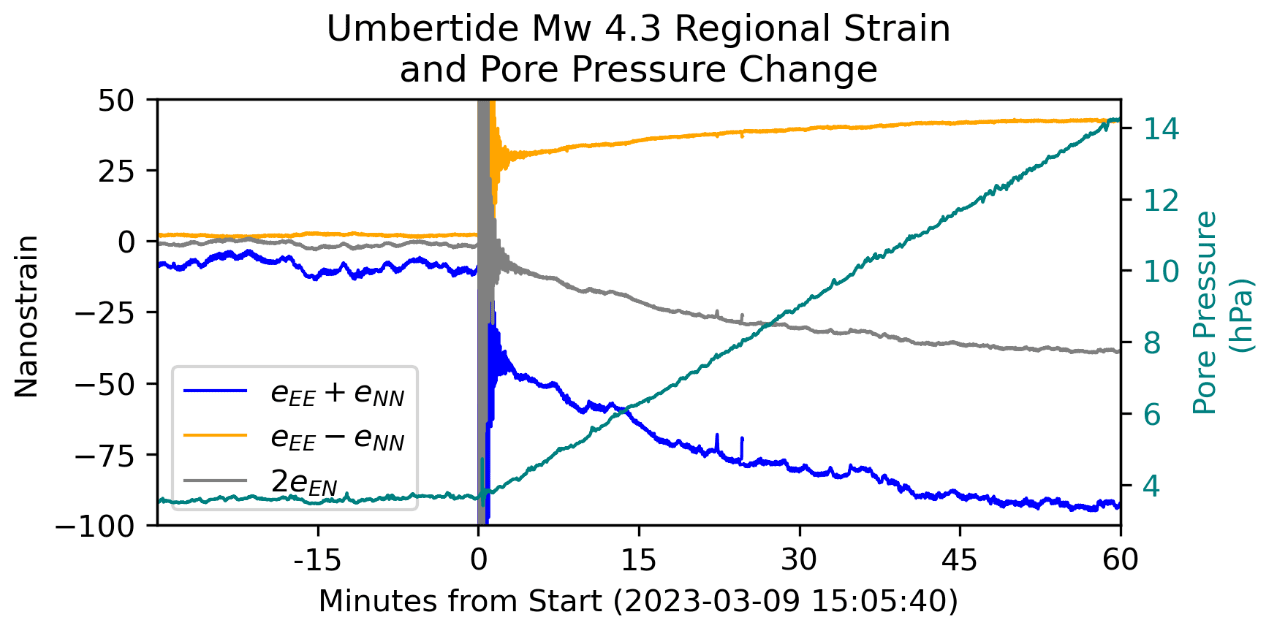
Figure 7 Demonstration of a high-rate (20 Hz) strain observations from the 9 March 2023 Umbertide M_w 4.3 earthquake at TSM3. The tidally calibrated regional strains are plotted for the areal (eEE + eNN), differential (eEE-eNN), and engineering shear (2eEN) strains according to the figure legend. The pore pressure data are plotted on the secondary y-axis in teal. Raw strain records and pore pressure data are downloaded from EarthScope.

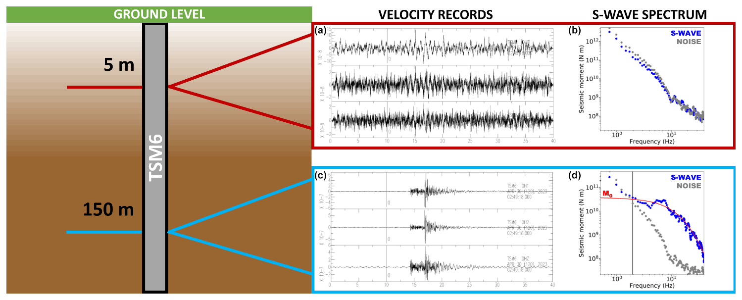
Figure 8 Small event recorded at the station TSM6 seismic instruments. (a) Three-component velocity signals recorded at the surface sensor. (b) Displacement spectrum of the expected (same time window observed in panel (c)) S-wave signal (blue circles) and of the noise (gray circles) recorded at the surface sensor. (c) As for panel (a), for the borehole sensor. (d) As for panel (b), for the borehole sensor; the black vertical bar is the minimum frequency used for the inversion, as defined by the SNR criterion of Supino et al. (2019). Event ID 34847211 (INGV catalog); the epicentral distance is 15.65 km, and the event depth is 1 km. The reference time in panels (a) and (c) is 30 April 2023 02:49:18 UTC.

It is important to mention that the raw gauge signals must be properly calibrated to accurately represent rock formation strain, and additional signal corrections can further aid in isolating non-tectonic signals, depending on the timescale of interest. The long-term trend is easily filtered or removed from the strain record. The measured tidal signals (Fig. 6) are useful for calibrating the four-gauge system response to rock formation strains in the east–north reference system by comparing the observed and modeled tides, which are approximately well-known (e.g., Canitano et al., 2018; Hodgkinson et al., 2013). These calibrations typically provide a more accurate characterization of tectonic strain than the standard manufacturer's calibrations (Hodgkinson et al., 2013; Roeloffs, 2010). The modeled tides can be removed from the time series, along with an estimated barometric pressure response derived from collocated surface atmospheric pressure data. Rain gauges at all stations and pore pressure transducers at TSM3, 4, 5, and 6 provide additional information related to strains induced by hydrologic changes (Figs. 6 and 7).

All strain data and data relevant to correcting the strain time series prior to geophysical analysis is available from the IRIS DMC (https://service.iris.edu/fdsnws/dataselect/1/, last access: 20 June 2024​​​​​​​). Metadata for proper calibration and corrections are currently hosted by UNAVCO for each station (https://www.unavco.org/data/strain-seismic/bsm-data/bsm-data.html, last access: 20 June 2024​​​​​​​).​​​​​​​

3.2 Seismometers

We report an example of a small earthquake (M_l = 0.7) in Fig. 8, detected by the 2 Hz seismometers deployed within the TSM6 borehole. We can appreciate how the event is barely visible at the surface sensor (Fig. 8a) but provides a high signal-to-noise ratio (SNR) signal at depth (Fig. 8c). Such a clean signal allows us to constrain the earthquake source parameter seismic moment from the S-wave displacement spectrum (Fig. 8d), computed with the probabilistic approach of Supino et al. (2019). The estimated moment magnitude is M_w = 1.0 ± 0.1.

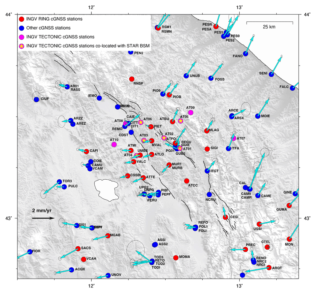
Figure 9 Map of the GNSS infrastructure. The cyan arrows show horizontal velocities, in an Apennines fixed reference frame for stations with more than 3.5 years of observation time span. Not all the blue stations are currently providing data.

3.3 GNSS antennas

Before the STAR project, the continuous GNSS (cGNSS) network across the Alto Tiberina fault zone was already dense with respect to the surrounding Italian regions (e.g., Devoti et al., 2017; Serpelloni et al., 2022), with average baselines among stations lower than the national average of 20 km. This is due to a relatively high number of GNSS stations, belonging to the INGV Rete Integrata Nazionale GNSS network (RING; http://ring.gm.ingv.it, last access: 20 June 2024), realized since the early 2000s (D'Agostino et al., 2009). When integrated with data from commercial and regional cGNSS networks, the spatial and temporal density allows for an estimate of high-resolution strain-rate measurements (e.g., Serpelloni et al., 2022), with important seismotectonic implications (Anderlini et al., 2016). However, it was necessary to improve the cGNSS network, which was originally designed as a linear array oriented in a direction perpendicular to the Apennine chain (D'Agostino et al., 2009). The implementation serves to increase both the spatial resolution of interseismic elastic coupling (see Anderlini et al., 2016) and our ability to detect small transient deformations of both tectonic and nontectonic origin (Gualandi et al., 2017; Mandler et al., 2021). Together with STAR, we benefit from the TECTONIC ERC project (https://cordis.europa.eu/project/id/835012, last access: 20 June 2024​​​​​​​) that gives us the opportunity to deploy an additional 10 GNSS instruments with the goal of improving the geometry of the RING network in the area (see Fig. 9). Six instruments have been installed in correspondence with the borehole strainmeters, with the GNSS antenna mounted on top of the well heads. An additional four sites have been installed following the semi-continuous scheme developed and described in Serpelloni and Cavaliere (2010). Once dismounted, only the geodetic marker remains fixed in the substrate (bedrock or building). The four semi-continuous stations are powered by solar panels, and data are delivered to the acquisition center through an LTE modem. For the six stations installed on top of the strainmeters, data are instead transmitted through satellite carriers.

Table 6 Description of the 10 continuous GNSS stations; the first six stations are installed on top of the borehole strainmeter well, whereas the other four stations (AT07, AT08, AT09, and AT10) are installed on bedrock or stable buildings. Note that AT07 was first realized in the framework of the RETREAT project (Bennett et al., 2012) and measured in repeated campaigns in 2005, 2006 and 2007. The first epoch reported in the table refers to the first measurement collected as a continuous station.

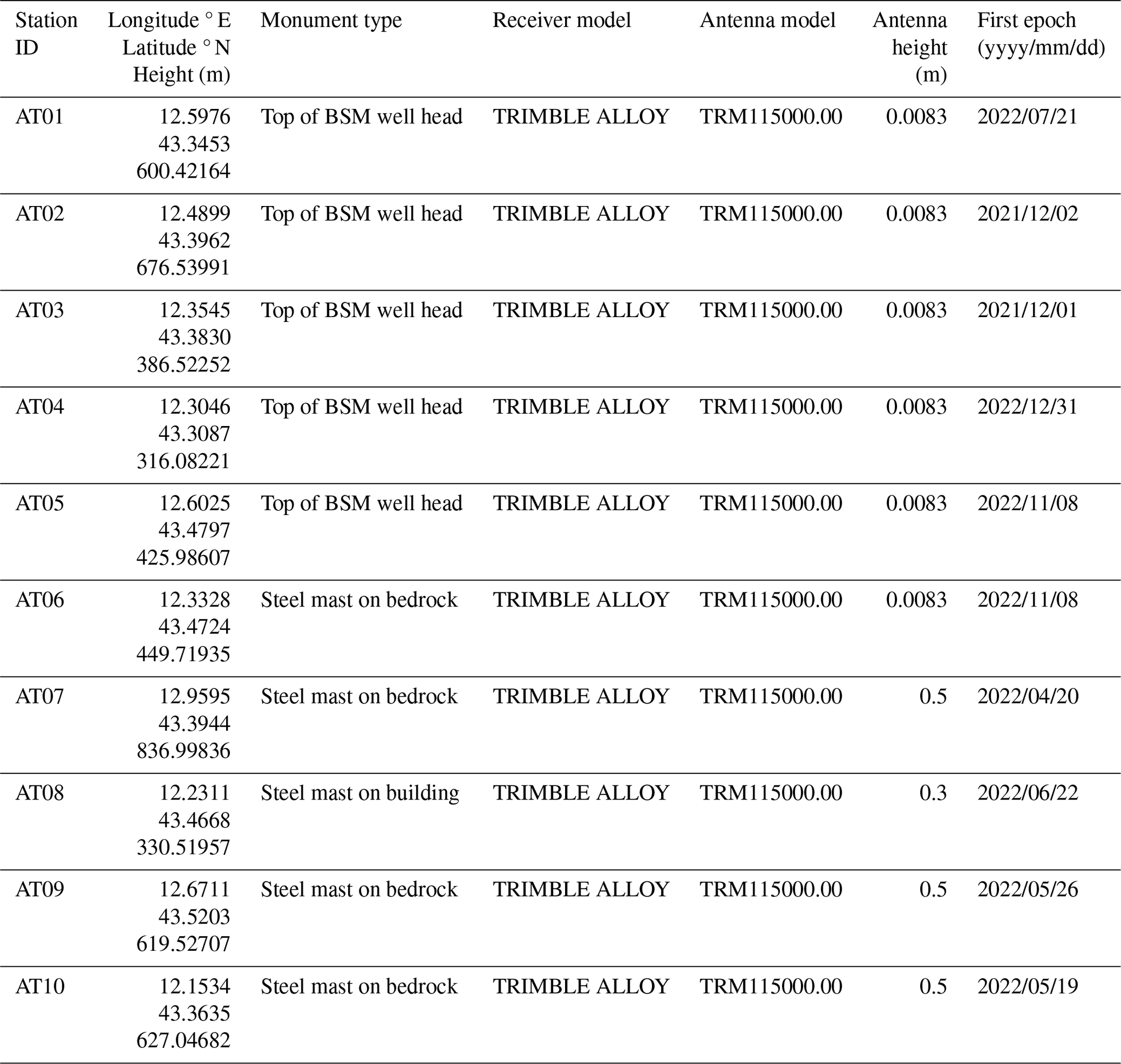
Table 6 lists the locations, GNSS instruments installed, and monument type for the 10 new cGNSS stations. Figure 10 shows photographs of the two types of installations adopted, while Fig. 11 shows the displacement time series obtained by processing the raw GNSS observations with the GAMIT/GLOBK software following the procedures described in Serpelloni et al. (2022). Given the still very limited temporal coverage (< 1.5 years) of the observations, the estimation of seasonal (annual, semi-annual, and multi-annual) components is still not accurate.

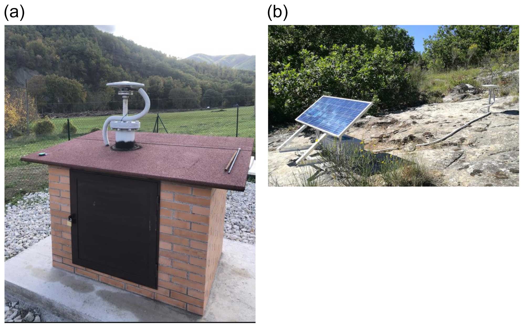
Figure 10 Photographs of GNSS station AT05 (a) installed on the well head at TSM3 site and GNSS station AT10 (b). AT10 is installed as a semi-continuous station on bedrock with a 50 cm tall antenna mount fixed on a ∼ 50 cm founded and epoxide geodetic marker.

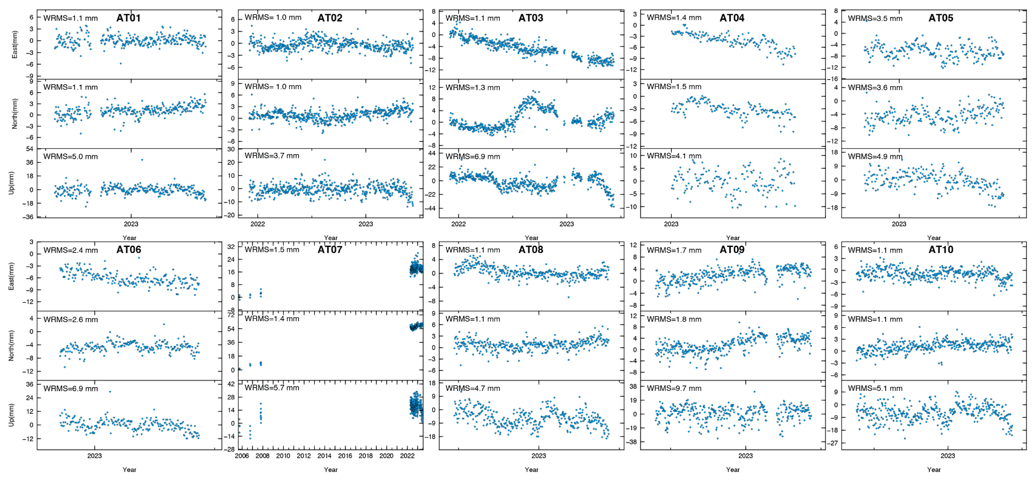
Figure 11 Displacement time series obtained from the analysis of GNSS observations using the GAMIT/GLOBK software, following the procedures described in Serpelloni et al. (2022). The horizontal components are rotated in a Eurasian fixed frame. Weighted root mean square (WRMS) values, from a linear fit of the time series, are indicators of daily repeatability for the east, north and vertical components.

3.4 Pore pressure and meteorological data

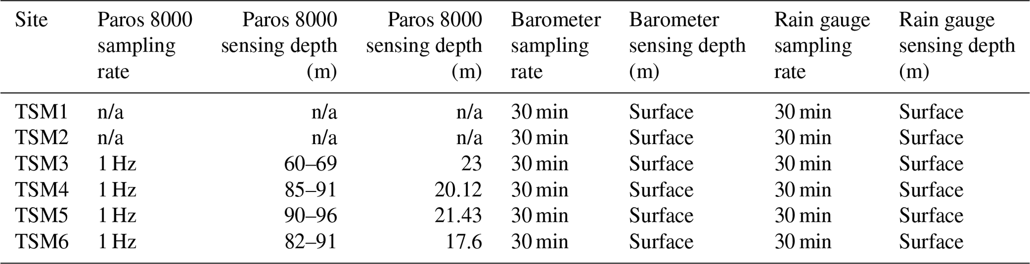
As previously mentioned, several additional sensors have been deployed at each station to collect data useful in generating post-processed corrections for the strainmeter data. In addition to the four strain gauges, the GTSM instrument records 30 min sampled environmental channels including barometric pressure and rainfall. Additionally, Paros 8000 Series pressure transducers are installed in four of the boreholes to record 1 sps pore pressure and temperature. The full complement of extra sensors at each station is described in Table 7.

Table 7 Location and sample rates of pore pressure and meteorological data. n/a – not applicable.​​​​​​​

Figure 12 Time series of availability of data per station.

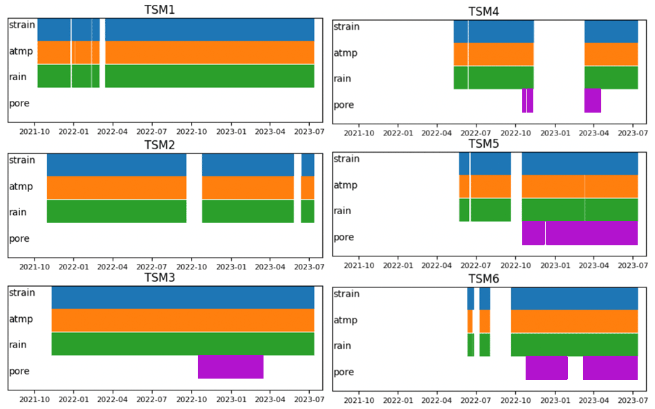
Pore pressure sensors were installed in a PVC pipe with a diameter of 5 cm, with a screened section (sampling depths listed in Table 4) sand-packed and capped with bentonite. Unfortunately, borehole conditions did not permit pore pressure installations at TSM1 and TSM2. The Paros sensors are connected to small board computers, which log 1 sps data into daily ascii files transmitted to EarthScope for archiving and distribution. The 30 min pressure and rainfall data are collected by the GTSM data logger and written into the daily bottle files. These data are translated to miniSEED and available as miniSEED or ascii formats from the EarthScope DMC. Figure 12 shows a time series of the currently available strain and correction data from each station.

4 Discussion and conclusions

The ATF is probably the best place in the world to understand the mechanisms and implications of the stress transfer process between seismic and aseismic fault segments at the local scale. By adding STAR to the existing TABOO NFO infrastructure, we realized one of the most complete and advanced system to investigate the complexities of fault slip processes at the local scale.

The ATF is an active low-angle normal fault that is directly related to the decades-long debate regarding the existence and mechanics of such structures in nature (e.g., Wernicke, 1995; Collettini and Sibson, 2001; Collettini, 2011).

The ATF is arguably the best location in the world for a BSM deployment targeting slip in a normal fault system because both steep and low-angle faults are present, and creep and episodic slip behavior are both known to occur (Chiaraluce et al., 2007; Hreinsdottir and Bennett, 2009; Gualandi et al., 2017; Anderlini et al., 2016). The greater ATF system is already among the best-instrumented fault systems in the world (e.g., Collettini and Chiaraluce, 2013; Chiaraluce et al., 2014). Consequently, the ATF has generated significant scientific interest internationally (e.g., MOLE workshop and report; EPOS NFO).

In addition to the ATF hazard problems of locally confined (even if crucial) importance, the STAR borehole array will allow us to address the global question of how aseismic slip relates to seismic slip. STAR data will also have implications for fault friction and crustal geodynamics that should be directly related to aseismic versus seismic fault slip more generally, including slip on transform faults, thrust and reverse faults, and subduction interfaces (e.g., Avouac, 2015). We anticipate that the strainmeter and other data we collect will have a broad impact on the global fault slip community, as testified by the international and definitively high profile of the colleagues ready to collaborate in the framework of the STAR scientific team. All data from TABOO are open to the international scientific community in standard format, available to inform studies of fault systems around the world. Data from STAR and other TABOO instruments will guide the interpretation of fault friction experiments from the laboratory (e.g., Collettini and Chiaraluce, 2013).