A comprehensive crosshole seismic experiment in glacial sediments at the ICDP DOVE site in the Tannwald Basin

Glaciers have shaped the Alpine landscape by carving deep valleys and depositing sediments to form overdeepened basins. Understanding these processes provides information on the evolution of the climate and landscape. One such overdeepened structure is the Tannwald Basin (ICDP site 5068_1) north of Lake Constance, which was formed by the Rhine Glacier in several glacial cycles. In order to study these sediments and their seismic properties down to about 160 m depth, we conducted seismic crosshole experiments between three boreholes, obtaining compressional (P) wave data. The P-wave data are generated by a sparker source and recorded by a 24-station hydrophone string. We present the data acquisition and review our approach for future optimization, suggesting a finer time sampling interval and a separate registration of borehole and surface receivers. Travel-time tomography of the P-wave first-arrival picks under geostatistical constraints yields initial subsurface models. The tomograms correlate well with cased-hole sonic logs and the lithology derived from the core of one of the boreholes. These results will be further investigated in future research, which will include full-waveform inversion (FWI) to obtain high-resolution subsurface models.

1 Introduction

Within the International Continental Scientific Drilling Program (ICDP) project 5068 “Drilling Overdeepened Alpine Valleys” (DOVE), we study overdeepenings in the Alps in order to understand climate and landscape evolution in Quaternary times. The valleys were excavated by glacial erosion and form elongated structures that usually correspond to the recent ice flow directions. Typically, these structures are quickly filled by various deposits. These deposits may then be eroded again by another glacial advance. The sedimentary infill of the valleys results in a complex system of aquifers with different permeabilities, so groundwater levels can vary greatly within short distances. Knowledge of the sedimentary structure is therefore crucial for water supply and shallow geothermal facilities. The rather soft sediments also play a decisive role in local site effects of earthquakes, which are common in the Alpine region. The DOVE project addresses these topics through a suite of geological, geochemical, geotechnical, and geophysical methods that heavily depend on the information obtained from cores as well as in and around the boreholes that were drilled for the project (Anselmetti et al., 2022).

At site 5068_1, the Tannwald Basin in southern Germany, not just one but three boreholes were drilled to conduct seismic crosshole experiments. Our seismic crosshole measurements are unique in that, to our knowledge, this acquisition geometry has never been used to investigate glacial sediments at depths down to about 160 m. However, the method is commonly used in the industry to investigate and characterize oil and gas reservoirs at depths greater than 500 m (Van Schaack et al., 1995; Bauer et al., 2005; Zhang et al., 2012; Liu et al., 2012) as well as geothermal sites (Martuganova et al., 2022; Gaucher et al., 2020); von Ketelhodt et al. (2018) applied the method to study aquifers in the upper 40 to 50 m by travel-time tomography.

Surface seismic methods, where the source frequencies are usually limited to below 200 Hz and strongly attenuated by the low-velocity weathering layer, which prevents high frequencies from penetrating the subsurface when shot at the surface, often lack the desired resolution. Crosshole seismic methods, which deploy high-frequency sources and receivers below the surface, can thus bridge the resolution gap between borehole methods (core analysis and logging) and surface seismic data. In addition, the transmission geometry samples horizontal travel paths, while surface seismic acquisition geometries predominantly treat vertical travel paths of seismic waves and local heterogeneities impair amplitude-variation-with-offset/angle (AVO/AVA) methods. This often prevents the study of complex geology, including the phenomenon of seismic anisotropy.

Here, we present the crosshole experiments we conducted in a glacially overdeepened basin of the Rhine Glacier. By a comprehensive discussion of the strengths and limitations of the data, we aim to encourage the application and improve the implementation of crosshole tomography in other projects. We are convinced that such measurements can provide crucial high-resolution information on sediment structures that cannot be derived from surface measurements. This is corroborated by the results of isotropic travel-time tomography, which can be linked to geological features observed in the lithology of the boreholes, demonstrating the value of the data.

2 Study site: 5068_1 (Tannwald)

Our study area is ICDP site 5068_1 in the Tannwald Basin and located about 45 km north of Lake Constance (Fig. 1a). The Tannwald Basin is a distal glacially overdeepened valley of the Rhine Glacier that is about 1 km wide and up to 250 m deep, and it is part of the Lake Constance amphitheater. According to Ellwanger et al. (2011), the Rhine Glacier incised into the Tertiary Upper Freshwater Molasse and the Upper Marine Molasse down below the fluvial base level during the Hosskirchian. Subsequently, the sediments transported in the glacial system refilled the basin during the Middle to Late Pleistocene. The study site lies beyond the maximum ice extent and thus beyond the terminal moraine of the Last Glacial Maximum (LGM) (Burschil et al., 2018).

Figure 1 (a) Location of the overdeepened Tannwald Basin and extent of the Rhine Glacier in the Quaternary in the northern Alpine Foreland (modified after Ellwanger et al., 2011). ICDP drill site 5068_1 is marked in red. (b) 3D view of the borehole trajectories and the locations of the 3C geophones at the surface. The circle has a radius of 28 m around borehole B.

Prior to drilling, the LIAG Institute for Applied Geophysics carried out intense pre-site surveys using surface seismic methods. These included five compressional wave (P-wave) seismic reflection lines distributed over the northeastern part of the basin. Using the high-resolution surface seismic data, Burschil et al. (2018) were able to characterize the sediments by reflection seismic imaging and facies characterization. A 3D survey at the drill site revealed additional faults and a glaciotectonic feature referred to as cuspate–lobate folding, which provides information on local stress regimes in the past (Buness et al., 2022). Based on the information from the seismic profiles, ICDP drilling site 5068_1 was selected.

Figure 2 Survey coverage of the crosshole experiments (adapted from Beraus et al., 2023). The source and receiver depths were limited by the groundwater level and the buoyancy of the drilling mud remaining in the boreholes after drilling. Note that plane AC was acquired in a separate survey as compared with the P-wave data from the shorter planes.

In comparison to the other DOVE sites, at site 5068_1 not just one but three boreholes (sites 5068_1_A, 5068_1_B, and 5068_1_C; hereafter referred to as A, B, and C) were drilled, all of which reached the base of the Quaternary overdeepened basin between 153 and 158 m depth (DOVE-Phase 1 Scientific Team et al., 2023b; Schuster et al., 2024). The boreholes are cased with a PVC pipe with a diameter of 80 mm. The backfill consists of bentonite and filter sand (DOVE-Phase 1 Scientific Team et al., 2023b). The boreholes are arranged in an isosceles triangle with short edges of 28 m that are oriented in N–S and W–E directions (Fig. 1b). This setup was found to be optimal for conducting seismic crosshole experiments in the glacial sediments. A detailed description of the drilling and the core recovered from borehole C can be found in Schuster et al. (2024) and DOVE-Phase 1 Scientific Team et al. (2023b, c). Cuttings from the flush drilling of boreholes A and B and core catcher information from the cored borehole C provided a preliminary lithology at each borehole location (Fig. 2; lithology: Bennet Schuster​​​​​​​, personal communication, 2021). The top layer consists of gravel, followed by mainly fines (silt/clay), interrupted by some sand layers in the cored borehole C, indicating that the sand was flushed out during the flush drilling of boreholes A and B. In addition, wireline logging data were acquired by LIAG during and after drilling (DOVE-Phase 1 Scientific Team et al., 2023b), providing information such as the borehole trajectories (Fig. 1b).

3 Seismic crosshole experiments

3.1 Data acquisition

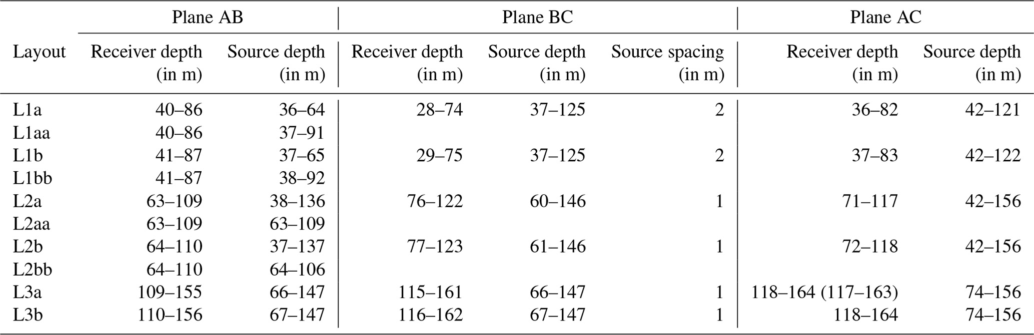
High-resolution P-wave data were acquired in all three borehole planes, i.e., AB, BC, and AC (Figs. 1b and 2), in two surveys. The first survey covered the shorter borehole planes between boreholes A and B and boreholes B and C, and the second survey covered the longer borehole plane between boreholes A and C. In both surveys, we used a sparker source in boreholes A and B, which requires a high-voltage power supply that is powered by a generator. The seismic waves were recorded with a 24-station hydrophone string. The hydrophones are omnidirectional pressure sensors which are spaced every 2 m along the receiver string. Both the source and the receiver string rely on them being placed below the groundwater level (GWL) (Table A1 in AppendixA) and being free to move laterally at depth, i.e., not coupled to the borehole walls. The shot and receiver depths are listed in Table 1. We shot eight times at each position to increase the signal-to-noise ratio (SNR). For the two short borehole planes, we chose a time sampling interval of 0.5 ms to ensure the required measurement progress. For the long plane between A and C, we decreased the time sampling interval to 0.125 ms.

Table 1 P-wave acquisition coverage of plane AB, plane BC, and plane AC. The source and receiver spacing within the layouts is 2 m. Layouts with double letters, e.g., “aa”, are referred to as the staggered scheme. The effective receiver spacing is 1 m. Note that for layout 3b of plane AC the planned receiver positions (in brackets) differ from the actual positions because the string was not moved downwards. The uncertainties of source and receiver positions are discussed in Sect. 3.3.

Furthermore, we deployed up to 112 three-component (3C) geophones at the surface. For the short plane measurements, we placed the stations every 1 m (plane BC) and every 2 m (plane AB) along the profiles connecting the wells to improve the polar coverage and, thus, the area of the borehole plane that is illuminated by the seismic waves. Additionally, we set up 48 receivers evenly distributed in a circle of radius 28 m around borehole B to sample the seismic wave field with azimuth. In the additional P-wave survey for plane AC, we deployed 56 three-component geophones along a line starting 1 m from the shot borehole A and going in the direction of the receiver borehole C with a spacing of 1 m. The surface station locations compiled from all surveys are shown in Fig. 1b, and the crosshole survey coverage is depicted in Fig. 2. We acquired approximately 40 GB of data in about 10 working days with a crew of three to four using borehole and surface receivers.

3.2 Raw data

The P-wave data have an overall excellent signal-to-noise ratio regarding environmental noise. However, they are also characterized by two distorting features: first by tube waves, which are often the most significant noise in crosshole sparker surveys (Daley, 1977), and second by aliasing (Fig. 3).

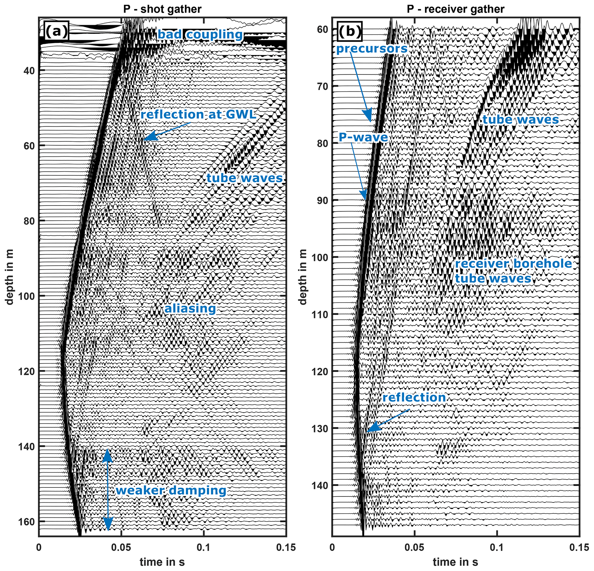
Figure 3 (a) Raw shot gather at 122 m depth with strong shot borehole tube waves. The top few stations were outside the water column in the receiver borehole C, resulting in long-period noise. (b) Raw trace-normalized P-wave receiver gather at 122 m depth with strong shot borehole tube waves and a weak receiver borehole tube wave.

The tube waves, which appear as linear noise in both the shot gathers and the receiver gathers, mask other late arrivals because of their high amplitudes. The steeply dipping events in the shot gathers (Fig. 3a) are associated with tube waves that originate at discontinuities in the source borehole and have velocities of about 1430 m s⁻¹, depending on the casing and formation discontinuities (Galperin et al., 2012). In the receiver gathers (Fig. 3b), the waves forming the linear events either travel through the subsurface and are then converted to tube waves at the receiver well or have already propagated as tube waves through the source well, radiated towards the receiver borehole, and are converted to tube waves once again. These waves can also be identified in the frequency–wavenumber (denoted fk) spectrum of the data (Fig. 4), where they appear as separate lines originating from k=0. Tube waves can be removed, e.g., by fk or τ−p filtering.

Figure 4 fk spectra of P-wave sparker data from plane BC showing tube wave energy, a wrap-around effect, and unusually dipping events originating at the minimum and maximum wavenumbers. For presentation purposes, we plot the spectrum to the power of 0.1 and apply a 95 percentile clip to the color map.

In order to prevent temporal aliasing, an anti-aliasing filter was applied during recording. However, it deteriorates the data quality in such a way that the P-wave first arrivals are not sharp but show precursors. These precursors are also offset-dependent and become stronger the shorter the source–receiver distance is. Spatial aliasing, caused by the source and receiver spacing of 1 m, however, could not be avoided, such that seismic events dip in two different directions simultaneously.

The fk spectrum of the field data from plane BC (Fig. 4) shows that most of the energy is concentrated in a triangle that is symmetrical to the frequency axis at k=0. However, a considerable amount of energy is aliased at about 270 Hz, resulting in a wrap-around effect in the fk spectrum. In addition, we can identify unusually dipping events in the fk spectrum that originate at the minimum and maximum wavenumbers.

Figure 5 Frequency spectra for P-wave sparker data from planes AB, BC (both panels a and b), and AC (c, d). (a, c) Normalized amplitude spectrum. (b, d) Normalized power spectrum. The solid lines represents the frequency content of the entire dataset; the dashed line represents that of the traces recorded for the shots at 122 m depth.

The frequency spectra from plane BC (Fig. 5a and b, red) show large peaks below 20 Hz. Another significant peak can be found at about 200 Hz. The cumulative spectrum, i.e., the normalized sum of the spectra of all shots, has its overall maximum at 345 Hz. Frequencies at 830 Hz, which corresponds to 83 % of the Nyquist frequency, are attenuated by −3 dB by the anti-aliasing filter applied during acquisition. Frequencies above 650 Hz already contribute less than 50 % to the signal energy. The normalized amplitude spectra of plane AB (Fig. 5a and b, orange) show a narrower peak at around 200 Hz and higher values at high frequencies. For plane AC (Fig. 5c and d, purple), where a finer sampling interval of 8 kHz was used, we observe several peaks below 500 Hz in the amplitude spectrum and another peak at about 1100 Hz. Frequencies above 1500 Hz contribute less than 30 % to the signal energy.

3.3 Discussion

In retrospect, we recommend focusing the P-wave surveys solely on the high-resolution imaging using horizontal travel paths and disregarding anisotropy investigations to reduce the number of shot positions required to obtain a proper angular coverage. Instead, a finer temporal sampling of at least 8 kHz would have ensured sharp phase onsets. For the longer plane between boreholes A and C, which was measured in a separate survey after the data were acquired in the short planes, the temporal sampling was reduced to 0.125 ms, which was sufficient to record the entire frequency range of the signal (Fig. 5) and thus sharp first arrivals.

To reduce the listening time, i.e., the time it takes to send the data to the computer, and with the intention of imaging by travel-time inversion methods as opposed to reflection imaging, we would reduce the total recording time to 800 ms. This would be sufficient to record first arrivals and reflections in our crosshole setting with short borehole spacings of 28 and 40 m (Liu et al., 2012). Later arrivals are too attenuated in the sediments to be visible in the data. Consequently, the recording time was adjusted in the acquisition of data in the plane between boreholes A and C. In addition, we would record the data at the surface seismic stations independently of the crosshole data, as the additional 336 channels are the main factor in the long listening time.

Although we additionally deployed 3C geophones along profiles at the surface between the boreholes, these data are not expected to be able to fully compensate for the limited angular coverage of the crosshole data due to the noise level caused by environmental noise. This includes factors such as vehicles passing directly by the site, trains commuting in the nearby river valley, and agricultural and forestry operations – all of which also cause a significant amount of downtime.

Regarding the noise identified in the fk spectra of the P-wave data, we interpret the unusually dipping events at the minimum and maximum wavenumbers in the fk spectrum as related to the interlacing of the receiver strings according to Watanabe et al. (2005). However, definitive verification is not possible, because we do no see systematic shifts in every second receiver depth. It seems reasonable to conclude that this is a display problem as a consequence of the temporal undersampling.

To avoid the spatial aliasing, a source and receiver spacing of 0.1 m would have been necessary. Thus, the depth errors of the borehole tools would be of a similar magnitude or even greater. These location errors include cable extension (up to 0.1 m), erroneous depth markers (up to ±0.1 m), and smaller errors (up to 0.05 m) due to clamping of the source and the receiver string. For the three to five deepest shot positions in borehole B, we estimate a position error of up to 0.5 m due to buoyancy caused by remaining drilling mud, depending on both the depth and the type of source and receiver.

4 Travel-time analysis

4.1 First arrival travel-time tomography and resolution test

In order to obtain preliminary subsurface models based on the P-wave first arrivals from the sparker data, we perform travel-time tomography. The method uses the phase picks and the acquisition geometry to invert the subsurface model. Synthetic travel times are computed based on Dijkstra's shortest path method, using secondary nodes to improve accuracy, as detailed by Giroux and Larouche (2013). Given the highly nonlinear nature of this geophysical inversion problem, an iterative optimization approach is employed to minimize the misfit between the field data and the simulated data. Here, we apply the damped Gauss–Newton algorithm with global regularization (Günther et al., 2006), which is implemented in the inversion code pyGIMLi (Rücker et al., 2017). It minimizes the objective function

$$\begin{array}{}\text{(1)}& \mathrm{\Phi }={\mathrm{\Phi }}_{\mathrm{d}}\left(\mathit{m}\right)+\mathit{\lambda }{\mathrm{\Phi }}_{\mathrm{m}}\left(\mathit{m}\right)\to \min ,\end{array}$$

where Φ_d(m) is the data misfit and where Φ_m(m) is the model sharpness. The parameter λ is the damping or trade-off parameter, which controls the relationship between data fit and model smoothness. Once the optimal model parameter updates, δm, have been identified, the algorithm updates the model on an unstructured mesh after each iteration step until it reaches the abort criterion. The latter is defined as the χ² value, which is construed as the mean of the sum of the squared data errors weighted by the misfit. Thus, reaching this criterion avoids both overfitting and underfitting of the data.

Since we expect a predominantly horizontally layered structure, we also apply geostatistical constraints to the inversion. This additional regularization uses the model covariance matrix to define a correlation ellipse, which is construed over the horizontal and vertical correlation lengths and the dip with respect to the horizontal direction (Jordi et al., 2018). Here, we choose a horizontal correlation length of 50 m and a vertical correlation length of 5 m for all three borehole planes without any dip.

We choose the initial model as the slowness, p, of the median apparent P-wave velocity, i.e., $p=\mathrm{1}/\mathrm{1935}$ m s⁻¹, derived from the data of the borehole plane AC. The damping or trade-off parameter, λ, is set to 2000 so that the inversion quickly reaches the target data fit, and any systematic pattern in the residuals is removed.

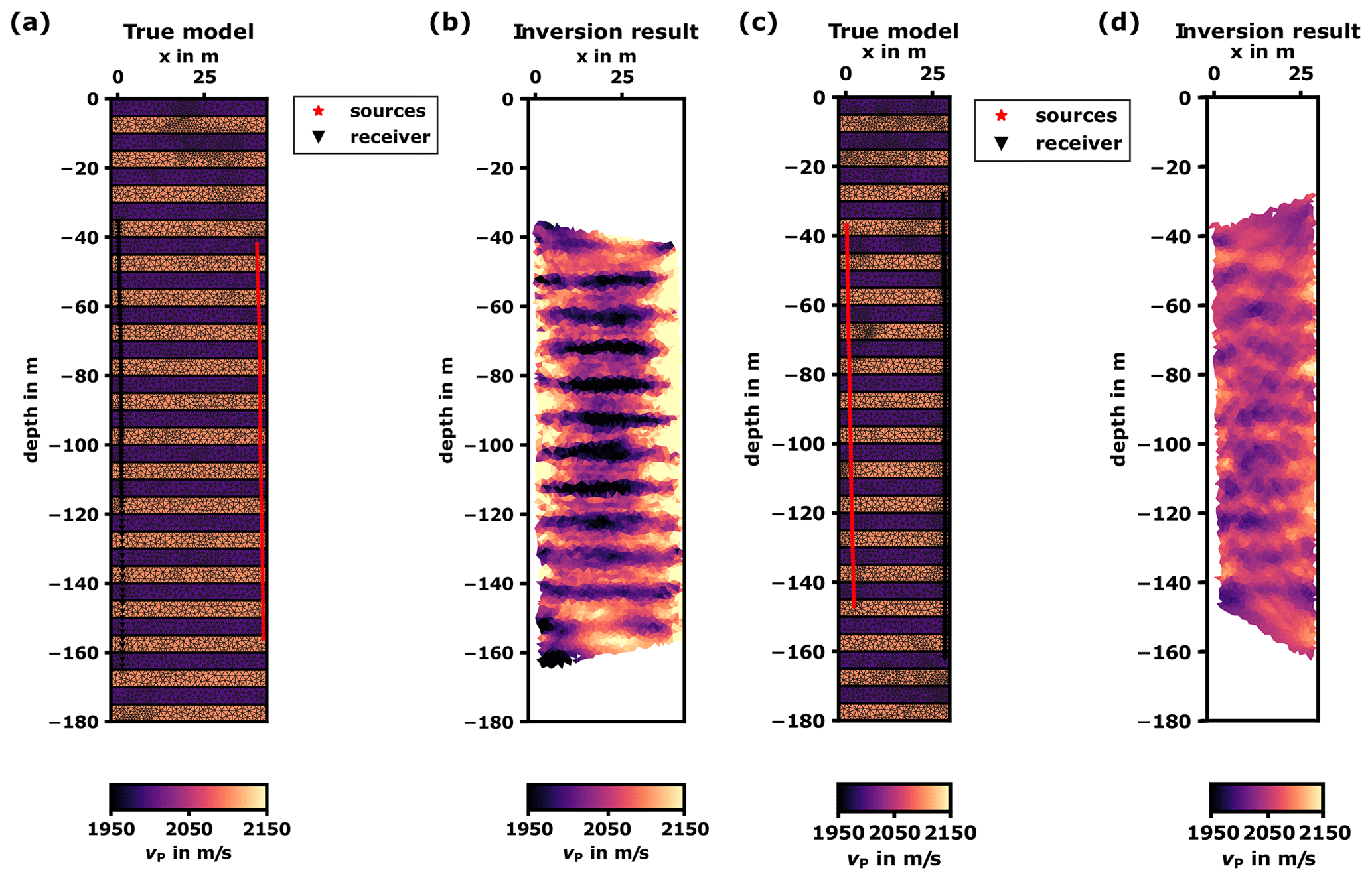
Figure 6 (a) Layered model for synthetic inversion test for plane AC. Fine lines show the modeling and inversion mesh. (b) Result of inversion of the forward modeled data from panel (a) including an absolute noise level of 0.125 ms. High-velocity layers appear thicker in the inversion result than low-velocity layers. (c) Layered model for synthetic inversion test for plane AC. Fine lines show the modeling and inversion mesh. (d) Result of inversion of the forward modeled data from panel (c) including an absolute noise level of 0.5 ms.​​​​​​​

Furthermore, we check the resolution of the tomography by means of a synthetic test model with 5 m thick layers (Fig. 6a and c), which differ in their velocity by 5 %. We forward calculate the travel times between the sources and receivers based on the model with a relative noise level of 1 % and an absolute noise level of 0.125 and 0.5 ms, corresponding to the respective temporal sampling interval and estimated picking error. Afterwards, we use a homogeneous initial model of 2050 m s⁻¹ and perform an inversion with the same parameters used to invert the field data.

4.2 Tomography results

The resolution test shows that 5 m thick layers could be well distinguished in plane AC using an unstructured mesh with a triangular area of 2 m² (Fig. 6a) if we assumed the actual picking error of this part of the dataset. The inverted high-velocity layers are thicker than the low-velocity layers (Fig. 6b), except in the central part at about 110 m depth, where the low-velocity layers are thicker. Furthermore, the layers extend all the way from the sources to the receivers. Nevertheless, a high-velocity zone is also recovered near the source positions. For plane BC (Fig. 6c), the layers are less well resolved in terms of the velocity contrast and their planar interfaces, which appear convex above 90 m depth (Fig. 6d). In general, layers that are above and below the sensor depth range are not resolved.

The inversion runs of the field data stop after a few iterations because they reach the abort criterion of χ²<1 (i.e., the inverted models explain the data within the assigned error of 0.5 ms). Figure 7 shows the obtained velocity distributions (tomograms) for all three borehole planes. The areas that remain white are those that are not traversed by the simulated seismic rays.

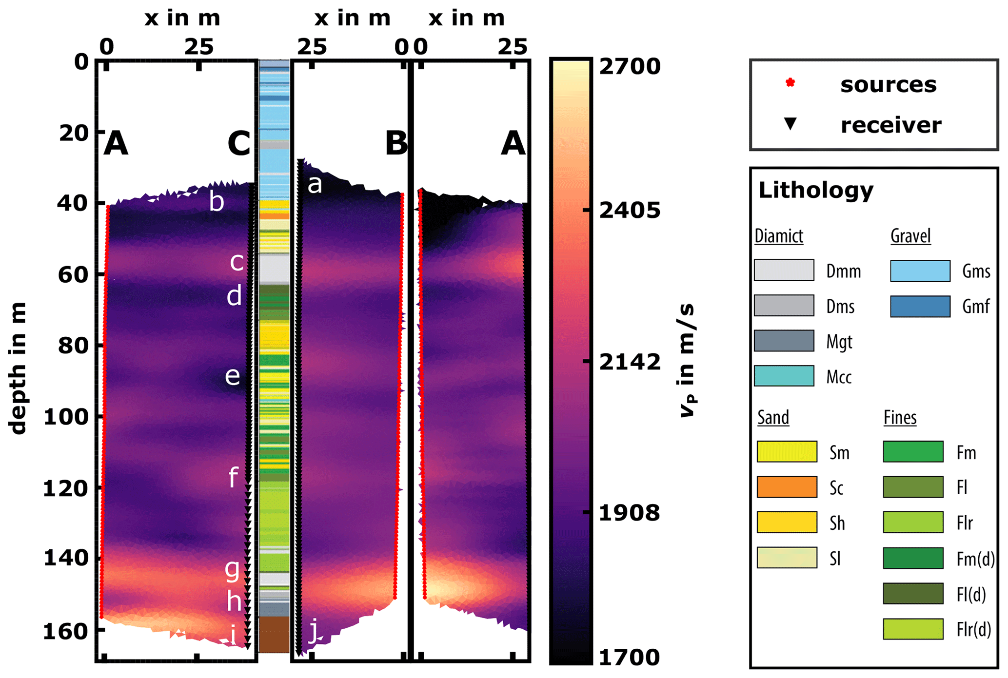
Figure 7 P-wave travel-time tomography velocity models and final lithology from the cored borehole C (Schuster et al., 2024). Receivers are marked by black triangles and sources by red stars. The x refers to the profile coordinate in Fig. 2.

All tomograms in Fig. 7 show a low-velocity (< 1800 m s⁻¹) structure at the very top of the model down to about 54 m (label a). In plane AC, this low-velocity zone is interrupted by a layer of a slightly higher velocity at about 40 m depth (b). Below this, we can identify an approximately 9 m thick layer with P-wave velocities of above 2000 m s⁻¹ that extends over all three planes (c). This is followed by another layer, about 5 m thick, with a velocity of about 1900 m s⁻¹ (d). At depths from about 75 m down to about 138 m, we see more layers, but they are not continuous in their extent or their velocities. Distinctive features in this depth range are a low-velocity zone at about 90 m depth, which is concentrated near borehole C and more pronounced in plane AC (e), and a high-velocity zone between 110 and 120 m depth on the same side of plane AC (f). Below 138 m, the tomograms show a high-velocity zone of about 2300 m s⁻¹ (g), followed by a layer, about 5 m thick, with velocities of 2200 m s⁻¹ (h). The former is more concentrated on the source sides of the short planes, while it is continuous in the long plane. The overall highest velocities are found at the bottom of the model with velocities of up to almost 2600 m s⁻¹ (i).

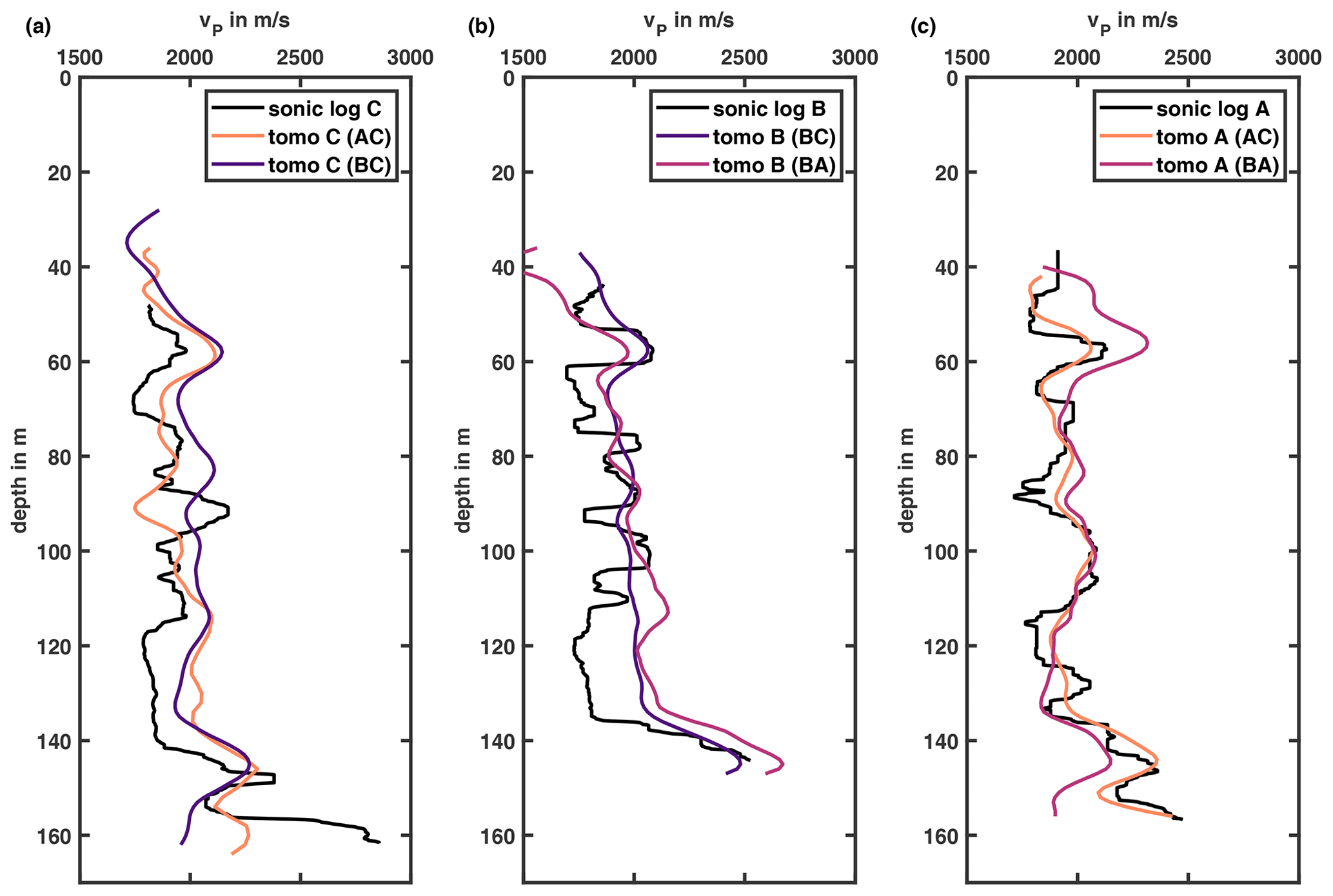
Figure 8 P-wave velocity profiles from smoothed wireline sonic logs vs. profile from travel-time tomography model for borehole C (a), borehole B (b), and borehole A (c).

From the tomograms of the field data inversion, P-wave velocity profiles are extracted along the borehole trajectories. They reasonably match the cased-hole sonic logs (Fig. 8), where the samples represent an averaged value over 0.5 m and which are smoothed over 5 m to make the datasets comparable. Along well A, the long-period trend is consistent. The profiles obtained from the long plane AC look like a further smoothed version of the sonic log. The profile from the shorter plane BA fits both the sonic log and the other profile at intermediate depth, but it has an overall trend from too fast to too slow from top to bottom. For borehole C, we observe a greater discrepancy between the tomography profiles and the sonic log, including an anticorrelation at about 90 m depth. There, the log indicates a high-velocity zone, while the tomograms show a low-velocity zone. Moreover, the velocity profiles from the tomograms exhibit a shift of approximately 200 m s⁻¹ towards higher velocities at depths of about 55 to 145 m. Furthermore, the low-velocity zone at depths from 114 to 144 m forms a less pronounced contrast than that observed in the sonic log. Additionally, the tomograms indicate a reduction in P-wave velocity at depths below 160 m, in contrast to the sonic log, which shows a strong increase of about 1000 m s⁻¹. The velocity variations along borehole B are considerably less pronounced in the tomograms than in the sonic log, so many minima and maxima cannot be identified and correlated. The tomography profiles also show a trend of increasing velocity with depth, which is not evident in the sonic log above 135 m. Nevertheless, the velocities are of a comparable magnitude.

4.3 Discussion

The resolution test confirms that we can distinguish layers of 5 m thickness with 5 % velocity difference. However, the high-velocity layers become thicker as the rays prefer to minimize the travel time. First-arrival travel-time tomography therefore favors arrivals from fast media. Thus, the low-velocity zones are sampled less densely with respect to the phase arrival picks and appear thinner, especially when the geostatistical regularization is applied, which effectively smooths the velocity field over 5 m in the vertical direction. Furthermore, the larger error estimate of the short planes results in a poorer resolution. However, the bending effect on the layers in the upper part cannot be observed in the field data tomography results of planes AB or BC.

Comparing the tomograms of the long plane AC with the two short planes AB and BC, the former shows more details, while the latter depict smoother velocity distributions. This can be explained by the higher picking accuracy of about a factor of 4 in plane AC, where a 4 times finer time sampling interval was chosen. The effect becomes evident when we compare the low- and intermediate-velocity zones above the high-velocity layer located at about 54 m (Fig. 7c). While the horizontally bedded sand layer (Sh) just below 40 m depth can be identified in plane AC as a zone of intermediate velocities (b), this is not the case in the two shorter planes. However, the weakly decreasing velocities in the layer towards borehole C might also indicate that the geostatistical regularization distributes the intermediate velocity information further than it actually reaches. The tomogram of plane BC also suggests that the layer might not continue into the direction of the plane but is interrupted by low-velocity material, which is not present in plane AC. This explanation is further supported by the tomogram of plane AB, where we see an intermediate-velocity zone close to borehole A but a low-velocity zone close to borehole B, indicating that the structure is interrupted halfway between borehole A and B, i.e., in the north–south direction. The complete absence of the intermediate-velocity zone, despite the correlation with the sand layer in the core, leads us to assume that the sand reaches only very little into plane BC and is smoothed out by the regularization. The shallow part of the tomograms from the short planes should be treated with care not only because of the coarse time sampling interval, but also because of the higher noise level at the shallow source and receiver positions. The high-velocity layer (c) below the just discussed shallow part clearly corresponds to a diamict found in the core at depths of about 54 to 63 m and extents over all three borehole planes. The next low-velocity layer (d) is associated with the fines found in the core. The discontinuities and velocity changes in depths from 75 to 138 m indicate a complex subsurface structure, which is confirmed by the alternating layers of sand and fines in the core lithology. Again, plane AC shows larger velocity contrasts, while the tomogram of plane AB depicts the layering down to about 118 m very well, including the layer boundary with the layers of only fines. The continuous high-velocity layer (g) at the bottom of the model correlates well with the massive diamict (Dmm). The thick low-velocity zone at the bottom of the short layers (j) is mostly an artifact of the smoothing, limited ray coverage, source mislocations due to the buoyancy of the remaining drilling mud in borehole B, and again inaccurate picks due to both the temporal sampling interval and the increased noise level because of the inert fluid at the bottom of the boreholes. In plane AC, this intermediate-velocity zone (h) is much thinner and correlates with the mélange (Mgt) “consisting of consolidated and unconsolidated molasse, sandstone, and siltstone fragments showing in situ crushing and brecciation” according to Schuster et al. (2024). The high-velocity layer at the very bottom (i) of plane AC eventually shows the molasse bedrock. A comprehensive sedimentological interpretation of the core lithology can be found in Schuster et al. (2024).

The overall trend of the profiles from the sonic logs and the tomographic models is similar (Figs. 7 and 8). The larger variations along boreholes C and B suggest that the formation close to those boreholes shows more variation than along borehole A. This near-field effect is well sampled by the sonic log, which inspects only a few decimeters of the formation around the borehole. The crosshole experiment, on the other hand, covers the plane between the boreholes and is sensitive to structures from the entire Fresnel volume with a radius of about 5 m. Furthermore, the geostatistical regularization with its horizontally extended correlation ellipse favors the inversion of layered structures and leads to smoothing of the velocity field. Differences in the velocity profiles obtained from different planes are related to picking inaccuracies, the geostatistical regularization, and location errors of the tools. The former is most obvious for borehole A, where the good-quality data from plane AC give an impressive fit to the sonic data, while the temporally undersampled data from plane BA show a larger deviation. In general, deviations of the velocity profiles at minimum and maximum depth are related to the reduced ray coverage in the tomography.

5 Conclusions and outlook

The crosshole data acquisition showed that the sparker source excites seismic waves with frequencies in the order of kilohertz (kHz). Therefore, the wave field has to be sampled very finely both in time and space, which increases the acquisition time and requires precise shot and receiver positioning. In this context, we discerned that the low-pass filter effect of the glacial sediments is much smaller than estimated from literature and anticipated during survey planning. We can clearly identify these effects in the data in the form of aliasing effects. Furthermore, the data are dominated by first-arrival P-waves and strong tube wave noise.

The travel-time tomography models, which show discontinuous layers in intermediate depths despite the application of a geostatistical regularization assuming horizontal layering, depict complex seismic wave fields indicating a heterogeneous basin infill. This is also reflected in the highly variable GWL over short distances of less than 40 m.

The velocity profiles extracted from the tomography models along the trajectory of the boreholes are in good agreement with the available sonic log data and the lithology of borehole C. However, we believe that this preliminary result can be further improved by full-waveform inversion (FWI), which considers not only the arrival time of a seismic phase, but also the entire waveform. This will require a thorough removal of the tube waves, yet it will increase the resolution to the decimeter scale, thereby bridging the gap between conventional surface seismic and core-scale information. Together with additional information from the core, the seismic subsurface models will be geologically interpreted.

Appendix A: Groundwater levels

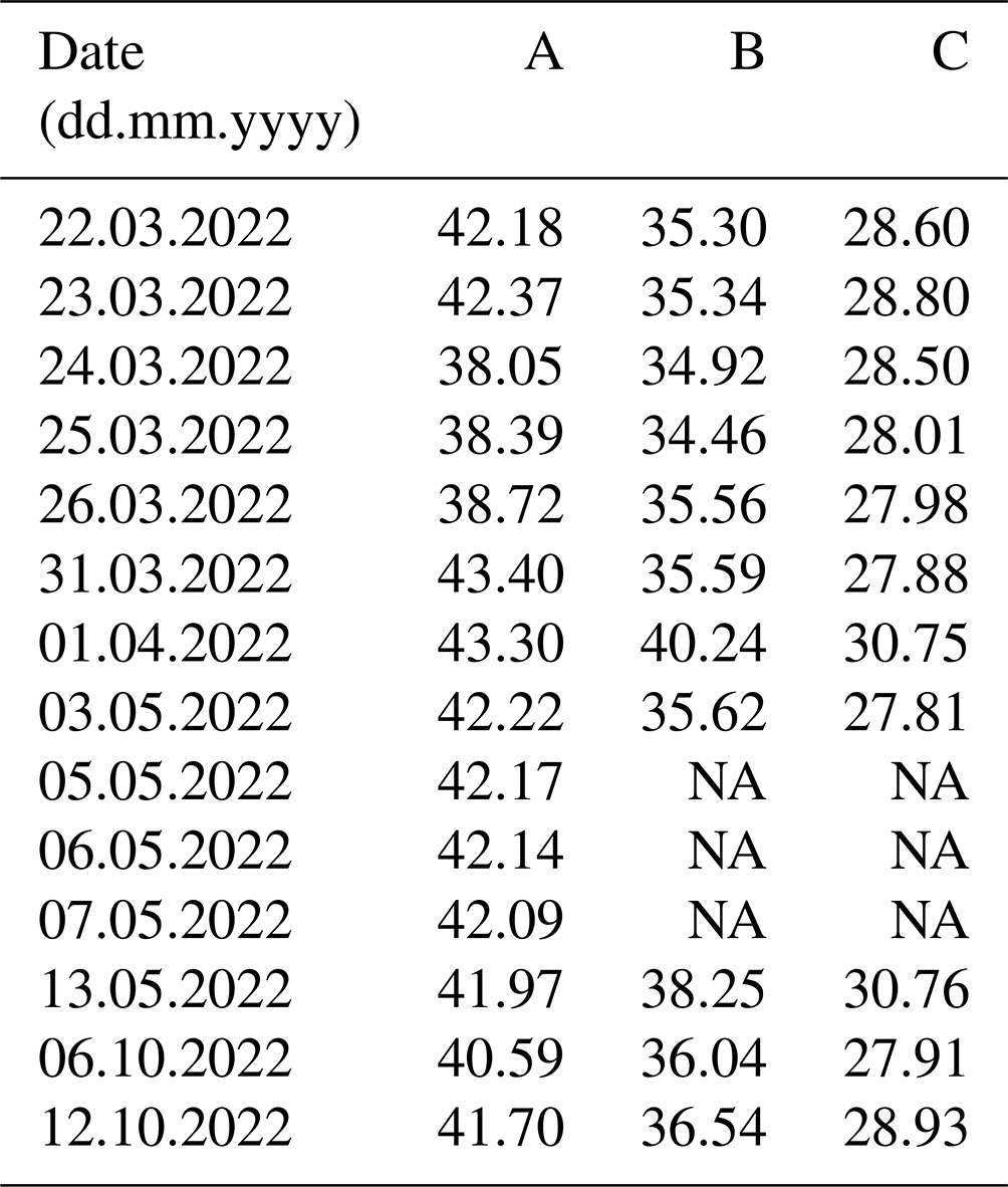
Table A1 Groundwater level (GWL) changes in boreholes A, B, and C during the time of the crosshole campaigns. Due to the instruments in the boreholes, the GWL in B and C was only measured at the beginning and the end of the survey. Note: NA represents not available.